![]()
![]()
This manual describes the Kappa language and details the usage of its tool suite.
Kappa is one member of the growing family of rule-based languages. Rule-based modelling has attracted recent attention in developing biological models that are concise, comprehensible, easily extensible, and allows one to deal with the combinatorial complexity of multi-state and multi-component biological molecules.
From the description of a system by the definition of a set of entities and the enumeration of their local rule of interraction, Kappa tools provide a framework to study statically and dynamically the system without ever enumerating all its reachable states (unless very explicitely asked to by users).
In Kappa, a mixture of entities is represented as a site graphs and temporal local transformations as rewrites.
First contact with Kappa as well as interactive model developement could occurs in the Kappapp available online and as downloadable software on main platforms. Intensive scientific usage should occurs by scripting around the command line tools or by using the Python client.
After a small teaser, this manual provides an exhaustive list of what can be done and how with the tools. It is not intended as a tutorial on rule-based modelling.
To get an idea of how Kappa is used in a modelling context, the reader can consult the following note Agile modelling of cellular signalling (SOS’08). A longer article, expounding on causal analysis is also available: Rule-based modelling of cellular signalling (CONCUR’07). See also this tutorial: Modelling epigenetic information maintenance: a Kappa tutorial.
See it really running in the online user interface by clicking on the try button on https://www.kappalanguage.org/.
A minimal Kappamodel looks like:
Lines 1-4 of this kappa file contain signature declarations. Agents of type C have two sites x1 and x2 whose internal state may be u (unphosphorylated) or p (phosphorylated). Line 11, rule 'ab.c' binds an A connected to someone on site x to a C.
There are two main points to notice about this model: A can modify both sites of C once it is bound to them. However, only an A bound to a B can connect on x1 and only a free A can connect on x2. Note also that x2 is available for connection only when x1 is already modified.
We try first a coarse simulation of events (10 times the number of agents in the initial system).
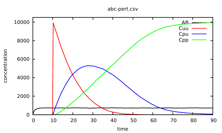
Plotting the content of the abc.csv file, one notices that nothing significantly interesting happens to the observables after 250s. So we can now specify a meaningful time limit by running:
which produces the data points whose rendering is given in Fig. 1.1.
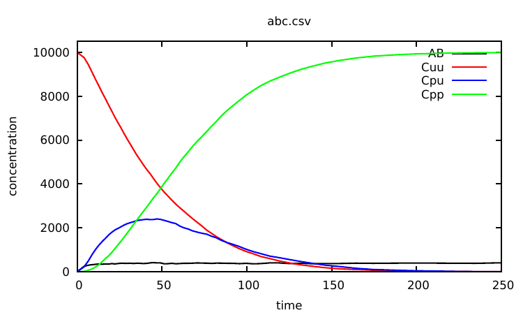
We will use variant of this model as a running example for the next chapter.
A model is represented in Kappa by a set of Kappa Files. We use KF to denote the union of the files that are given as input to a tool.
A KF is composed of a list of declaration. Declarations can be: agent and token signatures (Sec. 2.3), rules (Sec. 2.5), variables (Sec. 2.4), initial conditions (Sec. 2.6), intervention (Sec. 2.7) and parameter configurations (Sec. 5.4).
The KF’s structure is quite flexible. Neither dividing into several sub-files nor the order of declarations matters (for the exception of interventions and variable declarations, see respectively Sections 2.7 and 2.4 for details).
Comments works like in the C language. It can be used either by inserting the marker // that tells KaSim to ignore the rest of the line or by putting any text between the delimiters /* and */.
The following sections present formal grammars. Here are hints to read them. Terminal symbols are written in (blue) typed font, and stands for the empty list. An identifier Id can be any string generated by a regular expression of the type .
The state of the system is represented in Kappa as a sited graph: a graph where edges use sites in nodes. One must think sites as resources. At most one edge of the graph can use a site of a node (representing an agent in our case). Moreover, all the sites of an agent must have different names.
This leads to the property that an embedding between 2 sited graphs is completely defined by the image of one node. This is absolutely critical for the efficiency and we call this concept the rigidity of Kappa.
| Kappa_expression | ::= | agent_expression , Kappa_expression |
| agent_expression | ::= | Id(interface) |
| interface | ::= | Id internal_state link_state , interface |
| internal_state | ::= | | {.} | {Id} |
| link_state | ::= | | [.] | [n] | [_] | [#] | [Id.Id] |
The ASCII syntax we use to represent sited graphs follows the skeletons (describe formally in Table 2.1):
is written as A(x[.], y{p}[.], z{e0}[.]).
can be reprensented as A(x[23], y[4]{u}, z{e1}[.]), A(x[4], y{u}[95], z{e1}[.]), A(x[95], y{u}[23], z{e1}[.]).
Kappa strength is to describe transformations by only mentioning (and storing) the relevant part of the subgraph required for that transformation to be possible. This is the don’t care, don’t write (DCDW) principle which plays a key role in resisting combinatorial explosion when writing models.
If a transformation occurs independently from the state of a site of an agent, do not mention it in the pattern to match. The pattern A(x[.],z[.]) represents an agent of type A whose sites x and z are free but the sites y and z can be in any internal state and the site y can be linked or not to anything.
If the link state of a site does not matter but the internal state does, just mention it. An agent A whose sites x and z are free, y is in state u and z in state e2 is written as A(x[.],y{u},z{e2}[.]).
A state that is modified (by a rule that will be presented just below) always matter. For such situation, the symbol # (meaning “whatever” state) has been introduced.
In Kappa, in order to require a site to be bound for an interaction to occur, one may use the semi-link construct [_] which does not specify who the partner of the bond is. For instance, in the following instruction: %var: ’ab’|A(x[_]),B(y[_])|, the variable 'ab' will count the number of As and Bs connected to some agents, including the limit case A(x[1]),B(y[1]). It is sometimes convenient to specify the type of the semi-link, in order to restrict the choice of the binding partner. For instance, in the following instruction: %var: ’ab’|A(x[y.B]),B(y[x.A])|, the variable 'ab' will count the number of As whose site x is connected to a site y of B, plus the number of Bs whose site y is connected to a site x of A. Note that, this still includes the case A(x[1]),B(y[1]).
Remark Transformations on semi-links and links type induce side effects (effect on unmentioned agents/unmentioned site of agent) and can even do not make sense at all. What would mean to remove the link to A but not the link to B in the example above? Be careful when one use them.
Kappa tools can seek in the KF what agents are used, what sites they have and what states the sites are in but it is error prone: just make a typo once and the tools won’t complain and create a nonsens new agent/site/states...
To avoid that, Agent signatures can be defined and tools will then ensure that agents respect their signature.
Agent signatures list all the agents that will appear in the KF. They enumerate the name of interaction sites an agent has. They provide information about sites binding capabilities. They specify whether a site has internal state and if so give the possibilities.
A signature is declared in the KF by the following line:
according to an extention of the grammar given in Table 2.1. Linking states and internal states are space separated lists instead of being singleton. Site binding capabilities are specified by giving a list typed semi-links.
For instance, the line:
will declare an agent A with 3 (interaction) sites x,y and z, the site y possessing two internal states u and p (for instance, for the unphosphorylated and phosphorylated forms of y) and the site z having three possible states , and , sites x and sites y being able to bind (intra agent or inter agents).
Special case If no agent signature provides any site binding capabilities, constraints are released and any site of any agent is allowed to bind any site of any agent.
Algebraic expressions original purpose was to define kinetic rates for rules but many components of a KF will now implies algebraic expressions. Their syntax are defined in Table 2.2 (available symbols for variable, constants and operators are given in Table 2.3).
| algebraic_expression | ::= | variable |
| algebraic_expression binary_op algebraic_expression | ||
| tcbunary_op (algebraic_expression) | ||
| boolean_expression [?] algebraic_expression | ||
| [:] algebraic_expression | ||
The last item of the list is an if-expression. boolean_expression are described in Table 2.7. Think very carefully whether it is the correct thing to do before using it. Mechanistic conditions have to be expressed in rule bodies and not in rule rates!
| variable | Interpretation |
| [E] | the total number of (productive) simulation events |
| since the beginning of the simulation | |
| [E-] | the total number of null events |
| [T] | the bio-time of the simulation |
| [Tsim] | the cpu-time since the beginning of the simulation |
| 'v' | the value of variable 'v' (declared by using the %var: statement) |
| |t| | the concentration of token 2.5.5 t |
| |Kappa_expression| | number of occurences of the pattern Kappa_expression |
| inf | symbol for |
| unary/binary_op | Interpretation |
| [] | usual mathematical functions and constants |
| with |
Whatever symbols for link state [#] (for whatever state bound or not), [_] (for bound to some site), may also induce side effects when they are not preserved in the RHS of a rule, as in
or
To avoid mistakes, sites and states mentioned on the left must be exactly the same as sites mentioned on the right. Use the explicit “whatever” [#] state when needed.
Near any modified element, modification is specified. Created agents are postfixed by a . Degraded agents are postfixed by a . Site modifications are described by writing the new (linking or internal) state after the symbol inside the (curly/squared) bracket. Therefore, (inside squared brackets) means that the site becomes free, means that the site becomes part of link and inside curly brackets means that the new internal state of the site is .
Here are all the rules mentioned above (+1 extra) translated in this unambiguous notation:
Kappa rules are equipped with one (or two) kinetic rate(s). A rate is an algebraic expression (often simply a real number) evaluated as such, called the individual-based or stochastic rate constant, it is the rate at which the corresponding rule is applied per instance of the rule. Its dimension is the inverse of a time .
The stochastic rate is related to the concentration-based rate constant of the rule of interest by the following relation:
| (2.1) |
where is the volume where the model is considered, is Avogadro’ s number, is the arity of the rule (i.e. for a bimolecular rule).
In a modelling context, the constant is typically expressed using molars (or variants thereof such as , ), and seconds or minutes. If we choose molars and seconds, ’ s unit is , as follows from the relation 2.1.
Concentration-based rates are usually favoured for measurements and/or deterministic models, so it is useful to know how to convert them into individual-based ones used by KaSim. Here are typical volumes used in modelling:
A concentration of in a mammalian cell volume corresponds to molecules; molecules per cell.
A concentration of in a yeast cell volume corresponds to molecules; molecules per cell. The volume is doubled in a diploid cell.
A concentration of in a yeast cell volume corresponds to molecules; molecule per cell.
The table 2.4 lists typical ranges for deterministic rate constants and their stochastic counterparts assuming a mammalian cell volume.
| process | ||
| general binding | ||
| general unbinding | ||
| dephosphorylation | 1 | 1 |
| phosphorylation | 0.1 | 0.1 |
| receptor dimerization | ||
| receptor dissociation | ||
Using a Kappa rule of the form A(x[.]),B(y[.]) @ is not a good practice, where this rule could be applied in a context where A and B are sometimes already connected and sometimes disconnected. This would lead to an inconsistency in the definition of the kinetic rate which should have a volume dependency in the former case and be volume independent in the latter case (e.g. see Section 2.5.3).
This sort of ambiguity should be resolved, if possible, by refining the ambiguous rule into cases that are either exclusively unary or binary. Each refinement having a kinetic rate that is consistent with its molecularity. Note that in practice, for models having a large number of agents, it is sufficient to assume that the rule A(x[.]),B(y[.]) @ will have only binary instances. In this case, it suffices to consider the approximate model:
There exist systems where enumerating unary cases becomes impossible or where the approximation on binary instances is wrong. As an alternative, one should use the Kappa notation for ambiguous rules:
which will tell KaSim to apply the rule named 'my rule' with a rate for binary instances and a rate for unary instances.
The obtained model will behave exactly as a model in which the ambiguous rule has been replaced by unambiguous refinements. However the usage of such rule slowdowns simulation in a significant manner depending on various parameters (such as the presence of large polymers in the model). We give below an example of a model utilizing binary/unary rates for rules1 .
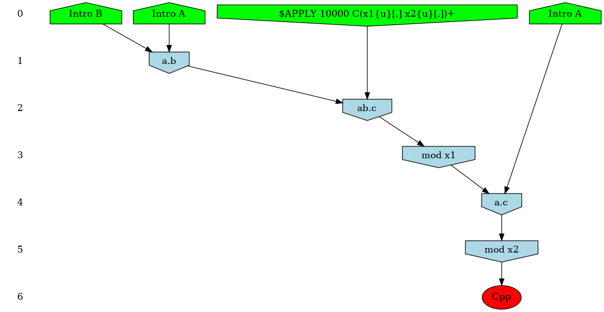
Notice at lines 10-12 the use of binary/unary notation for rules. As a result binding between freely floating agents will occur at rate 'k2' while binding between agents that are part of the same complex will occur at rate 'k1'. Line 21 contains a intervention that requires KaSim to stop the simulation after 10,000 events and output the list of molecular species present in the final mixture as a dot file (e.g. see Section 2.7) that we give in Figure 2.1.
For rules with unary rates, one can also specify a horizon. For example in the following rule:
the unary rate is applied only when the agents and are at a horizon (or closer), of each other. Horizon is an algebraic expression. It is always truncated to a positive integer during simulation. This feature can change in the future.
| rate_expression | ::= | algebraic_expression |
| | algebraic_expression {algebraic_expression:algebraic_expression} |
In Kappa, there can be a special treatment of entities that cannot bind anything: tokens. Tokens can only appear or disappear, they are typically used to represent small particles such as ions, ATP, etc.
Tokens may have a continuous concentration.
Token signatures are declared using a statement of the form:
It is possible to mix agents and tokens in hybrid rules (which may also be bi-directional). A hybrid rule has the following form:
Token expressions follow the grammar in Table 2.6.
| token_expression | ::= | algebraic_expression token_name |
| | token_expression , token_expression | ||
| token_name | ::= | Id |
Using Kappa hybrid rules, one may declare that an action has effects on the concentration of some particles of the system. For instance, a rule may consume atp, calcium ions, etc. It would be a waste of memory and time to use discrete agents to represent such particles. Instead one may declare tokens using declarations of the form:
One may then use these tokens in conjunction with a classical rule using the hybrid format:
When applied, the above rule will consume 0.2 atp token and produce 0.1 adp token. Note that as specified by the grammar given in Table 2.6, the number of consumed (and produced) tokens can be given by a sum of the form:
where each is an arbitrary algebraic expression (e.g. see Table 2.2) and each is a declared token. In the above hybrid rule, denoting by the respective evaluation of and , the concentration of token will decrease from and the concentration of token will increase from .
Importantly, the activity of a hybrid rule is still defined by |lhs|*r, where |lhs| is the number of embeddings of the LHS of the rule in the mixture, and does not take into account the concentration of the tokens it mentions. It is however possible to make its rate explicitly depend on the concentrations of the tokens using a variable rate.
Consuming tokens is strickly equivalent to producing tokens. All variations in amount of tokens can be written on the RHS of rules. This is what is done in edit notation when tokens are used:
The variations make clear that the simulator does not check that the consumed amount of token is available. It consumes tokens even if the quantity becomes then negative!
The initial mixture to which rules in the KF will be applied are declared as follows:
or:
where algebraic_expression is evaluated before initialization of the simulation (hence all token and Kappa expression values in the expression are evaluated to 0). This will add to the initial state of the model multiple copies of the graph described by the Kappa expression. The DCDW convention allows us not to write the complete interface of added agents (the remaining sites will be completed according to the agent’s signature). For instance:
will add 1000 instances of A in its default state A(x[.],y{u}[.],z{e0}[.]), 1000 instances of A in state A(x[.],y{p}[.],z{e0}[.]) and a concentration of 0.39 mM of calcium ions. Recall that the concentration of calcium can be observed during simulation by using the expression |ca2+|. As any other declaration, %init can be used multiple times, and agents will add up to the initial state.
Getting something out of a model is done like in lab experiment through intervention.
Each intervention directive is splitted in 4 parts:
There are 3 categories of intervention:
They are all described in detail below.
The general syntax is
for
and syntactic sugar detailed below is provided.
Boolean_expression and effect_list are defined by the grammar given in Table 2.7 (the operator rel can be any usual binary relation in and algebraic expressions are defined in Table 2.2).
There are 2 kind of clocks, an event based one and simulation time ones.
The event based one has the empty string for syntax: if nothing is written for clock, it uses the event based clock. It fires at the beginning of the simulation and every time a rule has just fired.
The time based one syntax is alarm float, it fires every amount of time unit given by the float (including at [T]=0).
For example %mod: alarm 2.3 [true] do $PLOTENTRY; repeat [true] will print a line in the data file every 2.3 time unit of simulation whereas %mod: |A()| > 1000 do $PLOTENTRY; repeat |B(x[_])| < |B(x[.])| will do it every event where there is more than 1000 A up to the first event where (there is more than 1000 A) and the number of |B(x[_])| becomes bigger than the number of |B(x[.])|.
When the conditions of several interventions that are tested at the same moment are satisfied simultanously, interventions are triggered in the order in which they have been declared in the KF. A intervention can only be fired once per event loop.
If the repeat keyword and the repeat condition are ommited, it is assumed that it is repeat [false] aka a one-shot intervention.
If the (pre)condition is ommited, it is considerated to be [true] unless both conditions are ommited and a clock is provided. In this case the implicit condition is [T] > 0 so that %mod: alarm 5.8 do effects is somehow a ’at’ operator. It means “do effects at [T] = 5.8”.
Special cases: simply adding or deleting agents Continuing with the ABC model, the intervention effect: $ADD n C(x1~p) will add instances of C with x1 already in state p (and the rest of its interface in the default state as specified line 4 of ABC.ka). Also the intervention effect: $DEL |B(x!_)| B(x!_) will remove all Bs connected to some agent from the mixture.
There are various ways one can use interventions to study more deeply a given Kappa model. A basic illustration is the use of a simple intervention to let a system equilibrate before starting a real simulation. For instance, as can be seen from the curve given in Fig. 1.1, the number of AB complexes is arbitrarily set to 0 in the initial state (all As are disconnected from Bs in the initial mixture). In order to avoid this, one can modify the Kappa file in the following way: one sets the initial concentration of C to 0 by deleting line 22. Now one introduces Cs after 25 t.u using the intervention: %mod: [T]=25 do $ADD 10000 C();.
The modified Kappa file is available in the source repository, in the model/ directory (file abc-pert.ka). Run a simulation again (a bit longer) by entering in the command line:
one obtains the curve given in Fig. 2.2.
Any variable between simple quotes can be updated during a simulation using a declaration of the form: %mod: ’Cpp’> 500 do $UPDATE ’k_on’0.0;
This intervention will be applied whenever the observable 'Cpp' will become greater than 500. Its effect will be to set the on rate of all binding rules to 0. Note that, according to the grammar given in Table 2.7, one may use any algebraic expression as the new value of the variable. For instance: %mod: ’Cpp’> 500 do $UPDATE ’k_on’’k_on’/100; will cause the on rate of all rules to decrease a hundred fold. Note that, it is possible to override the kinetic rate of a specific rule: in our ABC example, the declaration: %mod: ’Cpp’> 500 do $UPDATE ’a.b’inf; will set the kinetic rate of rule 'a.b' to infinity.
The intervention $STOP will interrupt the simulation. It returns the hand to the user if one run in interactive mode or terminates the run in batch mode.
The intervention $STOP "final_state.ka" will in addition produce a snapshot of the last mixture.
Advanced and/or experimental examinations are listed in chapter 5.
A snapshot is an instant photography of the current state of the mixture (a dump of the state at a given moment in the simulation).
A snapshot is suitable as an initial condition for a model. In the previous example, we let the system evolve for some time without its main reactant C in order to let other reactants go to a less arbitrary initial state. One may object that this way of proceeding is CPU-time consuming if one has to do this at each simulation.
An alternative is to use the $SNAPSHOT primitive that allows a user to export a snapshot of the mixture at a given time point as a new (piece of) Kappa file. For instance, the declaration: %mod: [E-]/([E]+[E-])>0.9 do $SNAPSHOT "prefix"; will ask KaSim to export the mixture the first time the percentage of null events reaches 90%. The exported file will be named prefix_.ka where is the event number at which the snapshot was taken. One may also use a string_expression to construct any prefix using local variables.
One may omit to define a prefix and simply type: %mod: [E-]/([E]+[E-])>0.9 do $SNAPSHOT; in which case the default prefix snap.ka will be used for naming snapshots.
If the name already exists, a counter will be appended at the end of the file to prevent overwriting. Snapshots can be performed multiple times, for instance every 1,000 events, using the declaration:
which results in KaSim producing a snapshot every 1000 (productive) events until the simulation ends.
Note that instead of producing Kappa files, one may use snapshot interventions to produce an image of the mixture in the dot/html format using the parameter by specifying the extention in the name skeleton (%mod: [E-]/([E]+[E-])>0.9 do $SNAPSHOT "snap.dot";).
The effect $PRINT string_expression >string_expression enables one to output values during a computation to:
For instance:
will ask KaSim to output the value of token A in a file "token_.dat" which changes at each new productive event, each time its value gets below 0.
The effect $PLOTENTRY outputs a line with the current value of observables in the data file. For example, %mod: repeat [E] [mod] 10 = 0 do $PLOTENTRY; until [false] will store the value of observables every 10 productive events.
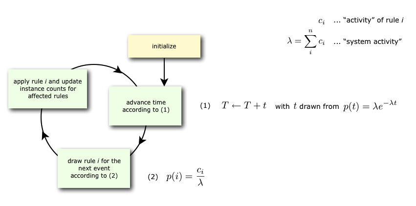
KaSim is a stochastic simulator of rule-based models [13, 12, 14] written in Kappa. KaSim takes one or several Kappa files as input and generates stochastic trajectories of various observables. KaSim implements Danos et al’s implicit state simulation algorithm [10] which adapts Gillespie’s algorithm [21, 22] to rule-based models.
A simulation event corresponds to the application of a rewriting rule, contained in the Kappa files, to the current graph (also called a mixture). At each step, the next event is selected with a probability which is proportional to the rate of the rule it is an event of. If there are no events, i.e. if none of the rules apply to the current state of the system, one has a deadlock. Note that a given rule will in general apply in many different ways; one says it has many instances. The activity of a rule is the number of its instances in the current mixture multiplied by its rate. The probability that the next event is associated to a given rule is therefore proportional to the activity of the rule. Rule activities are updated at each step (see Fig. 3.1). Importantly, the cost of a simulation event is bounded by a constant that is independent of the size of the graph it is applied to [10].
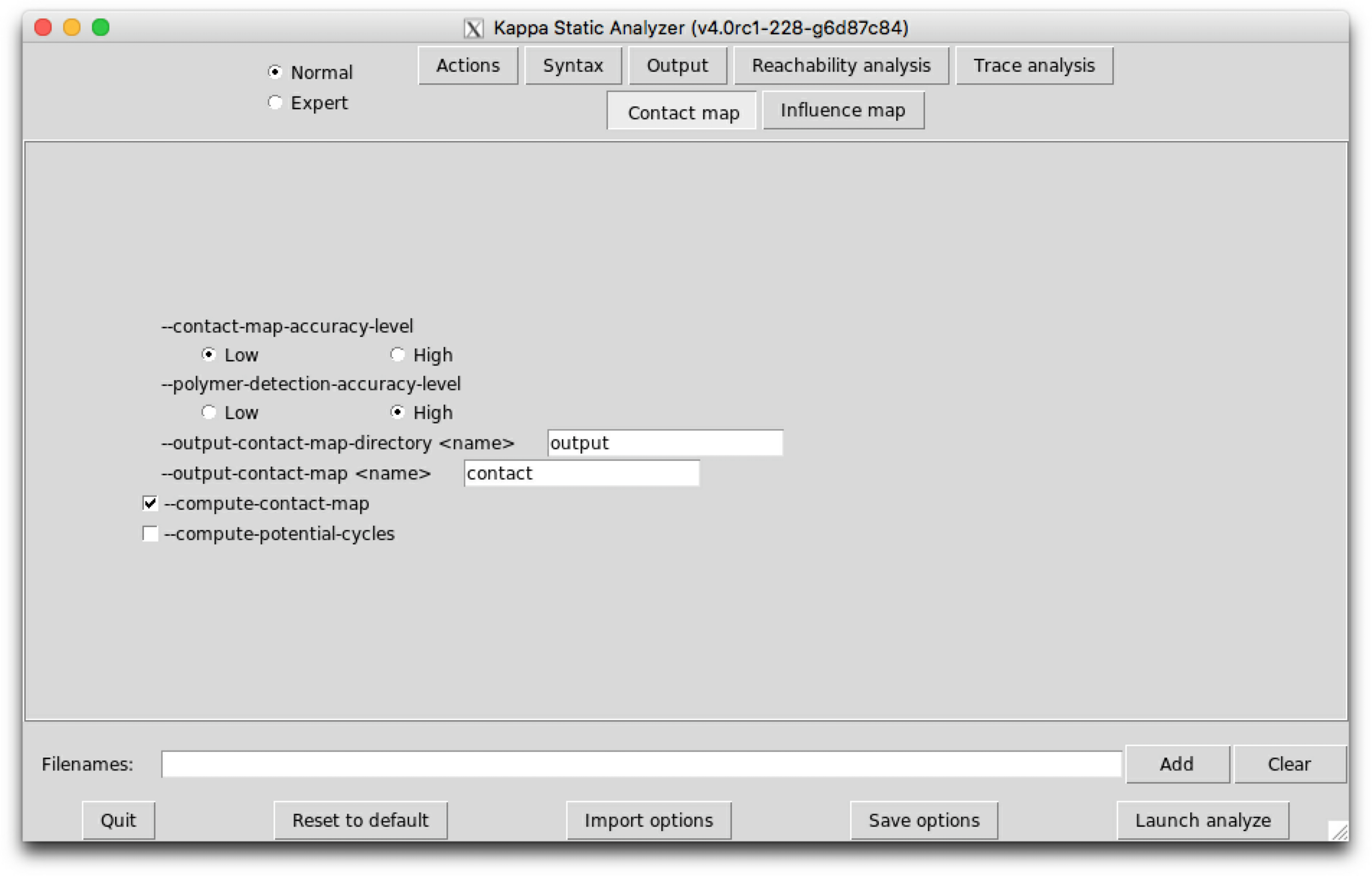
KaSa is a static analyser tool of rule-based models [13, 12, 14] written in Kappa. KaSa takes one or several Kappa files as input and some command line options to toggle on/off some specific static analysis. Currently, KaSa can compute the contact map and the influence map. It can perform reachability analysis [17, 11] as well.
A graphical interface is proposed to navigate through the various options and utilities of KaSa. The compilation of this interface requires labltk and, in particular, tk-dev.
KaDE is a tool to compile rule-based models [13, 12, 14] written in Kappa into systems of ordinary differential equations, or equivalently into reaction networks. It also supports some model reduction techniques, that may reduce the dimension of the ODEs (or the number of different bio-molecular species in reaction networks).
KaDE takes one or several Kappa files and uses some command line options in order to select a backend format, tune the semantics, and call some model reduction methods.
A graphical interface is proposed to navigate through the various options and utilities of KaDE. The compilation of this interface requires labltk and, in particular, tk-dev.
From a terminal window, KaSim can be invoked by typing:
where file_i are the input Kappa files containing the rules, initial conditions and observables (e.g. see Chapter 2). A simulation can generate several files that are described in the present chapter. One should really take advantage of the option -d so that these files all ends in a distinct directory.
In any case, a log called inputs.ka is generated. This is a valid Kappa file such that KaSim inputs.ka reruns exactly the simulation just ran outputing the exact same outputs (using the same pseudo random numbers!). First line of this file contains an uuid that is also present in any file output during the same run.
Tables 4.1 and 4.2 summarize all the options that can be given to the simulator.
Basically, one can specify an upper bound and a plot period either in simulated or bio-time (arbitrary time unit), or in number of events. Note that bio-time is computed using Gillespie's formula for time advance (see Fig. 3.1) and should not be confused with CPU-time (it is not even proportional).
Table 4.1 summarizes the main options that are accessible through the command line. Options that expect an argument are preceded by a single dash, options that do not need any argument start with a double dash.
Two key options are the plot period -p (how often you want a line in the data file) and the limit -l of simulation. These quantities can expressed in simulated time (the default) or in number of event (using -u event).
| Argument | Description |
| -u | Unit of options (time/event) |
| -l | Terminates simulation after |
| -initial | Starts the simulation at (data outputs convienience only) |
| -p | Plot a line in the data file every |
| -o file | Set the name of data file to file |
| Use the extension to determine format (’.tsv’, ’.svg’ or csv else) | |
| -i file | Interpret file as an input file name |
| (for compatibility with KaSim<= 3 and file names starting by -) | |
| -d dir | Output any produced file to the directory dir |
Table 4.2 summarizes the advanced options that are accessible through the command line.
The command:
will generate a file model.out containing the trajectories of the observables defined in the Kappa file model.ka. A measure will be taken every 1000 events in file model.out. The command:
will generate a file data.csv (default name) containing 1,000 data points of a simulation of 1.5 (arbitrary) time units of the model. The input Kappa file is split into four files containing, for instance, the initial conditions, init.ka, the rule set, rules.ka, the observables, obs.ka, and the interventions, pert.ka (e.g. see Chapter 2).
Simulations are interruptible by sending a SIGINT to the simulator. (The easiest way to send a SIGINT to a process is to press Ctrl-c in the terminal window it runs into.)
In batch mode, this stops the simulation. In other circumstances, it launches a toplevel in which one can either type:
A pause condition is a boolean expression (e.g. Section 2.7) under which the simulator will stop and fall back in the toplevel in order to allow a new interactive session.
The option -mode interactive interrupts automatically the simulation (and launches the toplevel) just after the initialization of the simulation.
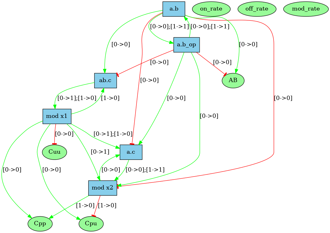
In our ABC example, adding the instruction: %mod: [true] do $TRACK ’Cpp’[true]; will ask KaSim to turn on causality analysis for the observable 'Cpp' since the beginning of the simulation, and display the causal explanation of every new occurrence of 'Cpp', until the end of the simulation. The explanation, that we call a causal flow, is a set of rule applications ordered by causality and displayed as a graph using dot format. In this graph, an edge r r' between two rule applications r and r' indicates that the first rule application has used, in the simulation, some sites that were modified by the application of the former. We show in Fig. 5.1 an example of such causal flow.
Causality analysis of the observable Cpp can be turned off at any time by using a declaration of the form: %mod: [T]>25 do $TRACK ’Cpp’[false];
Each time KaSim detects a new occurrence of the observable that is being tracked, it will dump its causal past as a graph using the dot format (see Fig. 5.1 above). The name of the file in which the causal flow is stored can be set by using the %def instruction (see Section 5.4).
In general, pure causal flows will contain a lot of information that modelers may not wish to consider. Indeed in classical flows, causality (represented by an edge between to rule applications in the graph) is purely local. Therefore a sequence only implies that an instance of rule caused an instance of rule which in turn created an instance of the observable . However, it does not imply that was "necessary" for to occur (for instance, might have been possible before but not after, and would be simply re-enabling ). It is possible to tell KaSim to retain only events that are more strongly related to the observable using two compression techniques (see Ref. [8] for formal details). Intuitively, in a weakly compressed causal flow one has the additional property that if an event is a (possibly indirect) cause of the observable, then preventing from occurring would have prevented the rest of the causal flow to occur (i.e. it is not possible to reconstruct a computation trace containing the observable with the events that remain in the causal flow). A strongly compressed causal flow enjoys the same property with an additional level of compression obtained by considering different instances of the same rule to be indistinguishable. Note that, causal flow compressions may be memory and computation demanding. For large systems it may be safer to start with weak compressions only.
The type of compression can be set using the %def instruction (see Section 5.4). For instance: %def: "displayCompression" "none" "weak" "strong" will ask KaSim to output 3 versions of each computed causal flow, with all possible degrees of compressions. Each causal flow is outputted into a file [filename][Type]_.dot where filename is the default name for causal flows which can be redefined using the parameter cflowFileName, Type is the type of compression (either nothing or Strongly, or Weakly) and is the identifier of the causal flow. For each compression type a summary file, named [filename][Type]Summary.dat, is also produced. It allows to map each compressed causal flow to the identifier of its uncompressed version (row #id), together with the production time and event number at which the observable was produced. It also contains information about the size of the causal flow.
As an example, consider the computation of causal flows between and using the declarations:
The above declaration will ask KaSim to analyze each new occurrence of 'Cpp' in that time interval. If new instances took place, then KaSim will have to compute causal flows. One may want to bound the number of computed flows to a certain value, say 10. One may do so using the combination of interventions and variables given below:
The first line is a declaration of an variable that is initially set to 0. Note that, the second line is a intervention that contains two simultaneous effects, the first one triggering causality analysis and the second one updating the value of variable to the current value of variable 'Cpp'. The last line stops causality analysis whenever time is greater than 20 or when 10 new observables have been found (the difference between the current value of 'Cpp' and ).
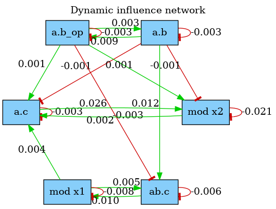
The dynamic influence network (DIN) is a powerful observation that tracks, on the fly, the influence that rule applications have on each others. It is dynamically generated and tracks effective impacts (positive or negative) at every rule application. The DIN can be computed using declarations of the form:
The result is a graph where a positive edge between rules and (in green) indicates an overall positive contribution of over . Otherwise, the sum of applications increased the activity of . Conversely, a negative edge (in red) will indicate that had an overall negative impact on the activity of . Note that, the importance of the influence between two rules can be observed by looking at the label on the edges that indicate the overall activity transfer (positive or negative) between the rules. The above declaration produces the network shown in Fig. 5.2. Note that, influence may vary during time, therefore the time or event limit of the simulation is of importance and will likely change the aspect of the produced map.
The effect $SPECIES_OFF tracks the occurrence of an observable. Each time a new instance of the observable appears, the species in which it occured is printed in a file. For example:
prints in the file "species.ka" a new line for each new occurrence of A(a!1), B(a!1) with the time of occurrence and the species in which it occurred.
Note that, this intervention can only be applied if the observable is a connected component.
KaSim permits users in a hurry to avoid writing agent signatures explicitly using the option --implicit-signature of the command line. The signature is then deduced using information gathered in the KF. Note that, it is not recommended to use the DCDW convention for introduced agents in conjunction with the --implicit-signature option unless the default state of all sites is mentioned in the %init declarations or in the rules that create agents.
The simulation algorithm that is implemented in KaSim requires an initialization phase whose complexity is proportional to where is the cardinal of the rule set and is the size of the initial mixture. Thus for large systems, initialization may take a while. Whenever a user wishes to run several simulations of the same Kappa model, it is possible to skip this initialization phase by creating a simulation package. For instance:
will generate a standard simulation of the abc.ka model, but in addition, will create the simulation package abc.kasim (.kasim extension is not mandatory). This package is a binary file, i.e. not human readable, that can be used as input of a new simulation using the command:
Note that this simulation is now run for time units instead of . Importantly, simulation packages can only be given as input to the same KaSim that produced it. As a consequence, recompiling the code, or obtaining different binaries, will cause the simulation package to become useless.
In the KF (usually in a dedicated file) one may use expressions of the form:
%def: "parameter_name" "parameter_value"
where tunable parameters are described in table 5.1 (default values are given first in the possible values column).
| parameter | possible values | description |
| Simulation | ||
| "maxConsecutiveClash" | "2" or any integer | number of consecutive clashes |
| before giving up | ||
| square approximation | ||
| "T0" | float | simulation starting time |
| (outputs convienience only) | ||
| "seed" | any positive integer | pseudo-random number |
| generator seed | ||
| Outputs | ||
| "traceFileName" | string | outputs simulation trace |
| in the given file | ||
| "outputFileName" | string | data file name |
| "plotPeriod" | number then optionally | interval between |
| "events" | plot lines | |
| Causality analysis | deprecated | please use KaStor |
| "displayCompression" | any combination of | type of compression |
| "none", "strong", "weak" | ||
| "cflowFileName" | "cflow", any string | file name prefix for causal flows |
| "dotCflows" | "no", "html" | generate causal flows in html |
| "yes", "dot" | generate causal flows in dot | |
| "json" | generate causal flows in json | |
| Pretty printing | ||
| "dumpIfDeadlocked" | "no","yes" | snapshot when simulation |
| is stalled | ||
| "colorDot" | "no", "yes" | use colors in dot format files |
| "progressBarSymbol" | "#" or any character | symbol for the progress bar |
| "progressBarSize" | "60" or any integer | length of the progress bar |
An agent can have counters, which are sites storing a positive integer. When declaring an agent, each counter has to be assigned a min and a max value. For instance, the agent %agent: A(x,c:1 += 4,d:0 +=2) has two counters, named and , which range from to , and from to , respectively.
| signature_expression | ::= | Id(sig) |
| sig | ::= | Id internal_state_list, sig Id counter_test counter_modif , sig |
At initialisation, an initial value for the counter has to be specified.
In rules, all counter tests have to be in the LHS, while the counter modifications in the RHS. A counter test can do three things: (i) check that the counter value is equal to a positive integer; (ii) check that the counter’s value is greater than a positive integer or (iii) declare a variable, to which the counter’s value is assigned. The variable can then be used in the rate constant.
A counter modification increments or decrements the original counter value. In the following table, and both and are integers.
| counter_expression | ::= | Id counter_test counter_modif |
| counter_test | ::= | : n :> n :> variable |
| counter_modif | ::= | : i |
If the counter goes negative, the compilation stops with an error. If the counter goes up beyond its declared maximum value, the simulation stops with an error.
From a terminal window, KaSa can be invoked by typing the following command line:
where file_i are the input Kappa files containing the rules, initial conditions and observables (see Chapter 2).
All the options are summarised as follows:
Order in options matters, since they can be used to toggle on/off some functionalities or to assign a value to some environment variables. The options are interpreted from left to right.
More options are available in the OCaml file KaSa_rep/config/config.ml and can be tuned before compilation.
The graphical interface can be launched by typing the following command line:
without any option.
There are five different areas of importance in the graphical interface:
Contextual help is provided when the mouse is hovered over an element.
The interface will store the options that are checked or filled and the order in which they have been selected. When launched, the analysis interprets these options in the order they have been entered.
Some options appear in several sub-tabs. They denote the same option and share the same value.
Importantly, options are saved automatically under various occasions. Thus, it is possible to restore the value of the options before the last reset, before the last quit, or before the last analysis.
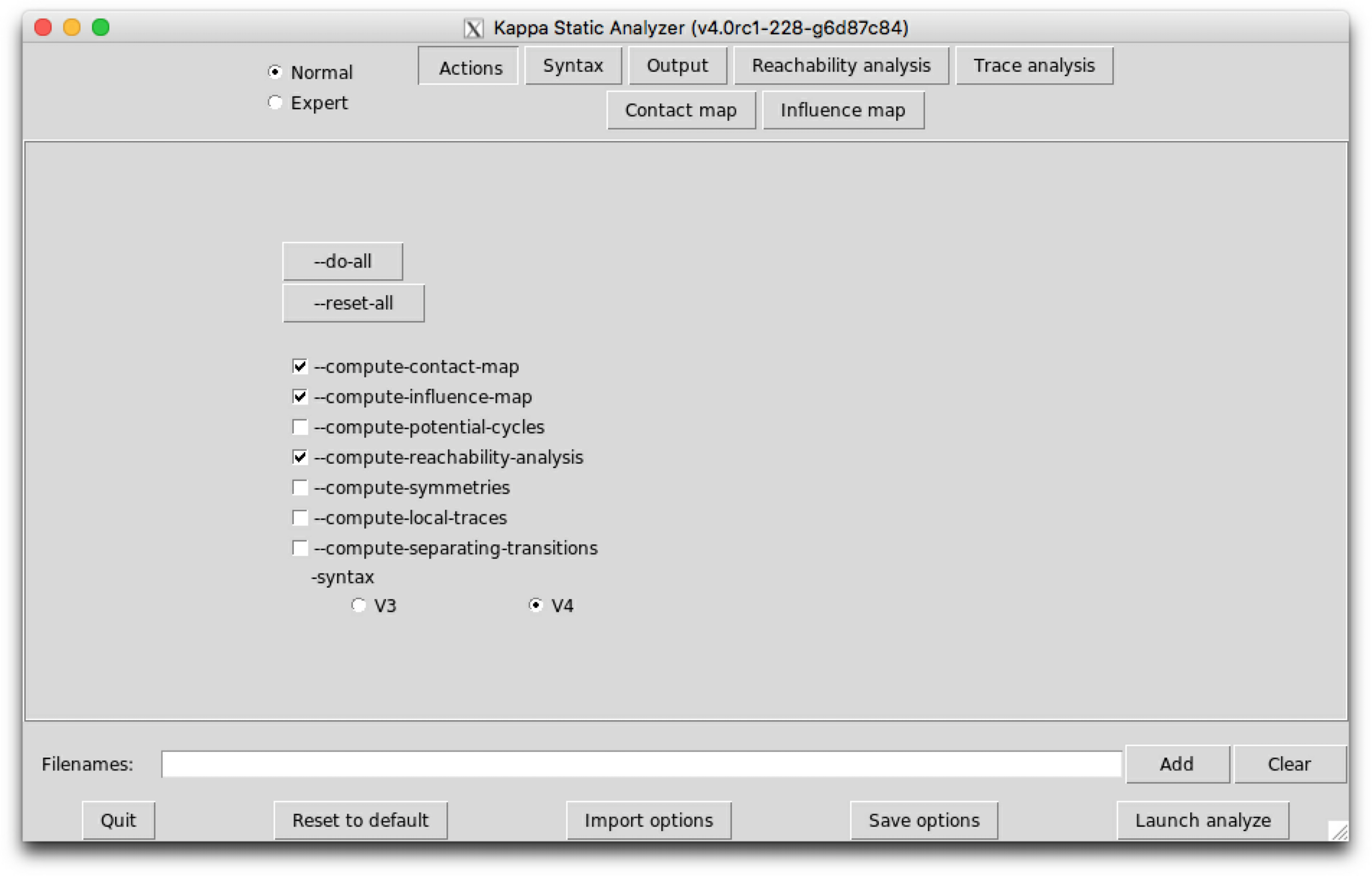
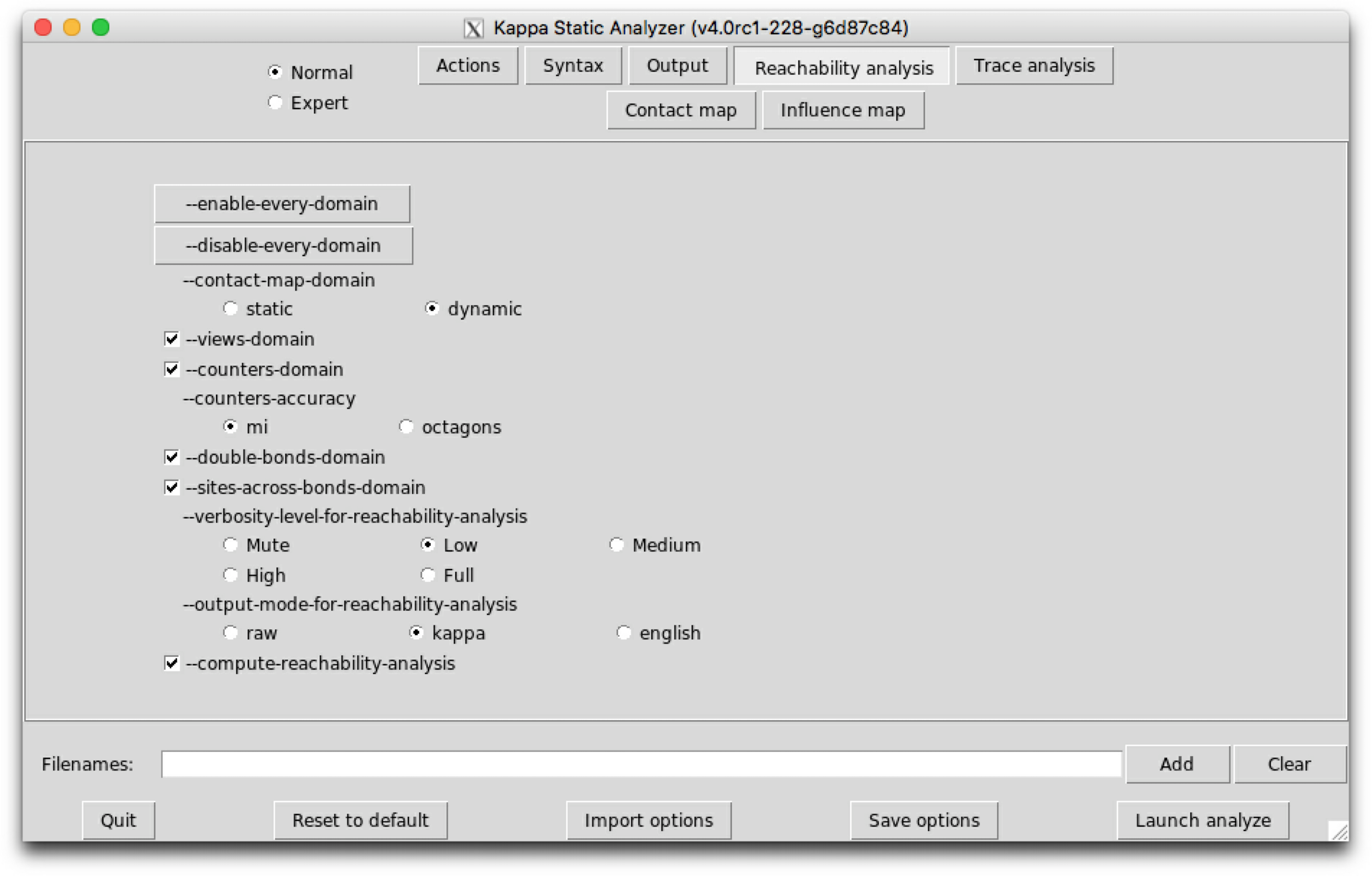
The sub-tab Actions (see Fig. 6.1) contains the main actions which can be performed.
The following options are available:
Lastly, a switch allows to select the version for Kappa syntax for the input file, among version , V3, and version , V4.
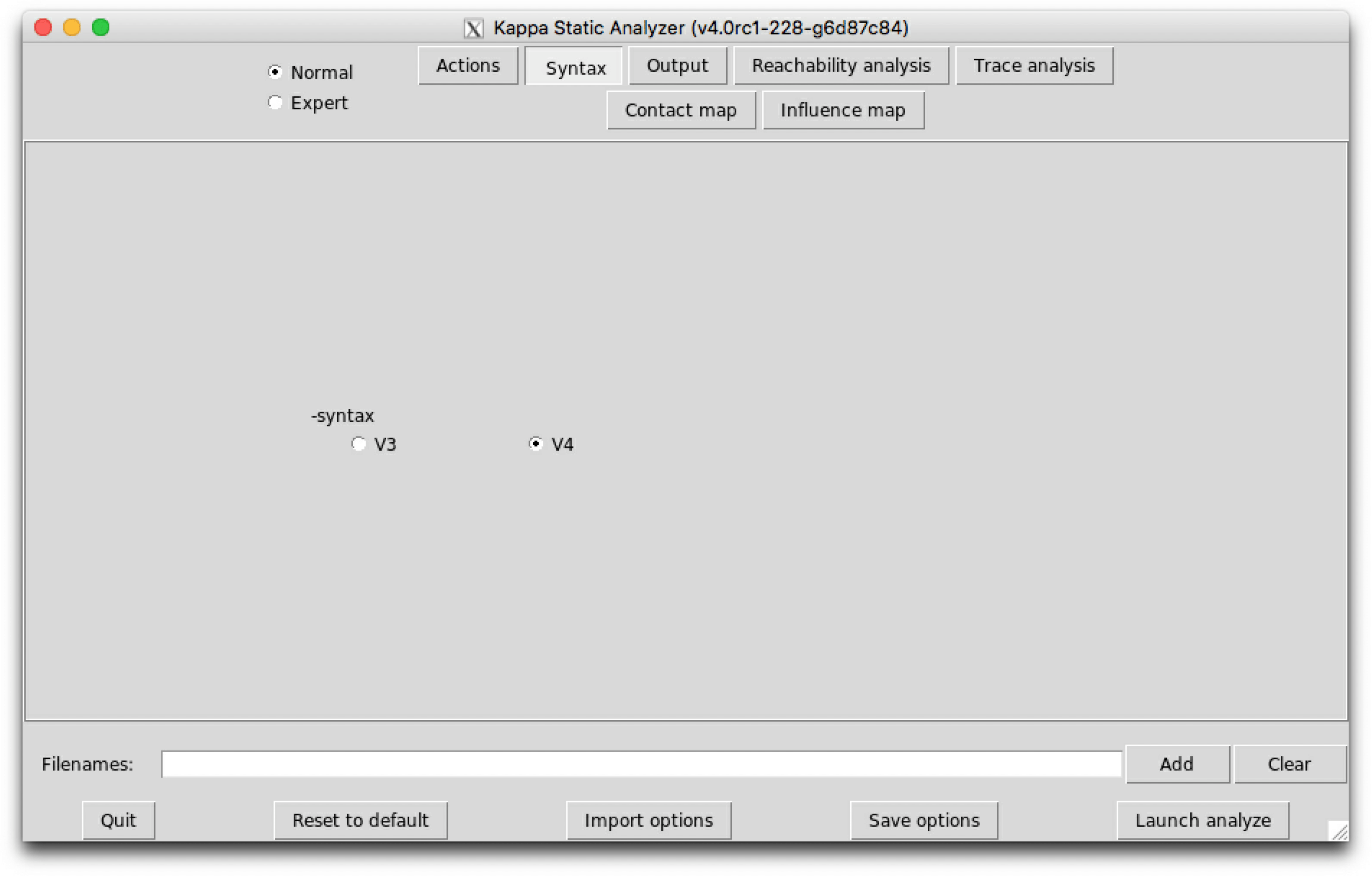
The sub-tab Syntax (see Fig. 6.2) contains the switch to select between the version 3, V3, and the version 4, V4, of Kappa syntax.
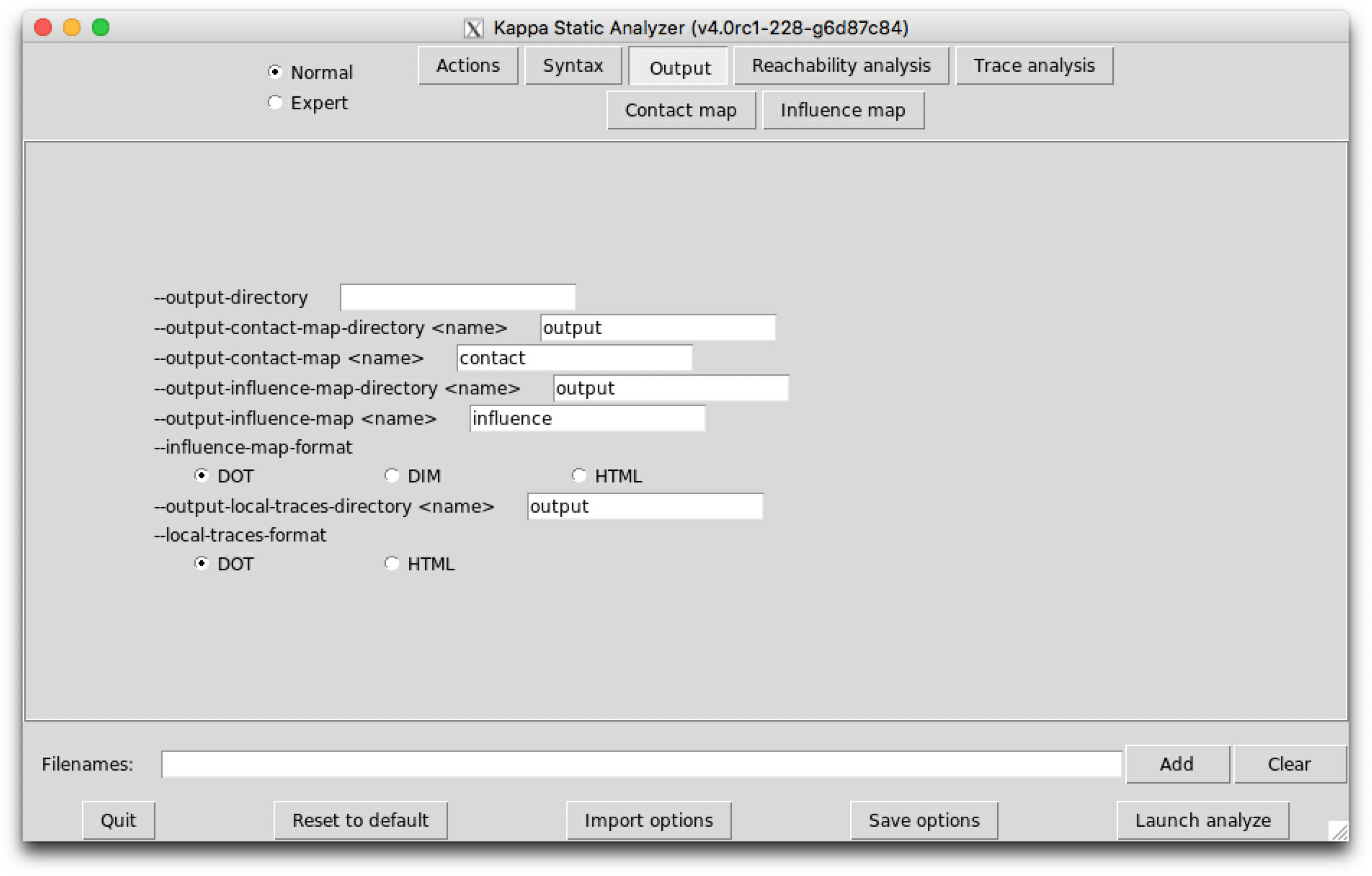
The sub-tab Ouput (see Fig. 6.3) contains the names of the output files and their format.
The following options are available:
When a file already exists, it is overwritten without any warning.
Reachability analysis aimed at detecting statically properties about the bio-molecular species that may be formed in a model. Knowing whether, or not, a given bio-molecular species may be formed in a model is an undecidable problem [24]. Thus, our analysis is approximate. Indeed, it computes an over-approximation of the set of the bio-molecular species that can be reached from the initial state of the model, by applying an unbounded number of computation steps. As formalized in [11, 20], the abstraction consists in:
The analysis takes into account also the chemical species that may be introduced in a intervention.
The classes of properties of interest are encoded in so called abstract domains, which can be independently enabled/disabled. The whole analysis can be understood as a mutual recursion between smaller analyses (one per abstract domain), that communicate information between each other at each step of the analysis. We took the same scheme of collaboration between abstract domains as in [6].
As an example, we consider the following model:
Typing the following command line:
will perform the reachability analysis on the model reachability.ka.
We obtain the following result:
This result is displayed in the standard output, and it is made of six parts.
The first two parts provide an enumeration of dead rules and dead agents. The next parts display what we call refinement lemmas. A refinement lemma is made of a precondition (on the left of the implication symbol) that is a site graph, and a postcondition (on the right of the implication symbol) that is a list of site graphs. Each site graph in the post-condition is a refinement of the precondition (the position of agent matters: the -th agent in the precondition corresponds to the -th agent in each site graph in the postcondition, but site graphs in a postcondition may have more agents than the site graph in the corresponding precondition). The meaning of a refinement lemma is that every embedding between its precondition into a reachable state can be refined/extended into an embedding from one site graph in its postcondition into the same reachable state. This way, a refinement lemma provides an enumeration of all the potential contexts for the precondition.
We now detail the seven different parts:
In our example, we notice that the rule ‘obs’ can never be trigered.
In our example, there are no dead agent.
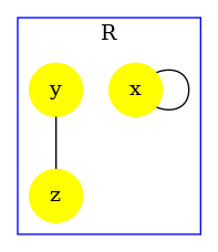
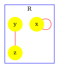
In our example, the site cr of R may be free, or bound to the site n of an agent R.
In our example, the states of the sites c, cr, n, and x of R are entangled with a relational property (othewise, we would have elements in the post-condition).
This abstraction aimed at capturing information about protein transportation. It is quite common to model the location of a protein as the internal state of a fictitious site. With such an encoding, it might be important to ensure that two connected proteins are always located in the same location. This abstraction focuses on this kind of properties.
It might be interesting to know whether a protein can be bound to another protein twice simultaneously, and whether a protein can be bound to two instances of a same protein simultaneously. This abstraction [20] captures this kind of constraint. It can be used to prove that some proteins do not polymerize.
In our example, when a R has its sites cr and c bound, they are necessarily bound to the same instance of R. The same statement holds for the sites cr and n.
KaSa is inferring the range of counters.
There are no counter in our previous example. Let us consider the following one:
Typing the following command line:
we get in the section ‘Properties of counters’ of the output what is prompted in Fig. 6.11. KaSa has inferred that the counter c is ranging from to . There is no information on counter d since its value has no lower bound and no upper bound.
By default, KaSa is using a relational numerical analysis based on a product between interval analysis [5] and affine relationship analysis [23]. The product is approximate. It used a decision procedure described in [16].
Other abstractions for counters are available for pedagogical purpose. For instance, the following command line:
will provide no property for counters (e.g. see Fig. 6.12). KaSa has failed in bounding the range of the counter c
Now we describe the options that are available on this sub-tab.
The option --compute-reachability-analysis can be used to switch on/off then reachability analysis.
The option --enable-every-domain can be used to switch on every abstract domain, whereas the option --disable-every-domain can be used to switch off every abstract domain.
The option --contact-map-domain impacts the way side-effects are handled with during the analysis. In static mode, we consider that every bond that occurs syntactically in the initial state, in the RHS of a rule, or in an introduction directive of a intervention, may be released by side-effects. In dynamic mode, only the bond that has been encountered so far during the analysis are considered.
The option --views-domain can be used to switch on/off the views domains that combine the non-relational analysis and the relational analysis.
The option --counters-domain can be used to switch on/off the analysis of the potential range of counters.
The option --counter-accuracy can be used to select the abstraction for the potential range of counters. The domain mi consists in an approximate reduced product between interval analysis [5] and affine relationships [23]. The reduction between these two domains, is obtained by applying the decision procedure that is described in [16]. The domain octagons infer a range for each variable, each sum and each difference among two variables. Although both domains have the same complexity, the product between intervals and affine constraints is more appropriate in the case of counters, since usually the state of more than two variables have to be related.
The option --double-bonds-domain can be used to switch on/off the analysis of potential double bonds between proteins.
The option --site-across-bonds-domain can be used to switch on/off the analysis of the relations among the states of the sites in connected proteins.
It is possible to get more details about the computation of the analysis by tuning the verbosity level of the view analysis:
When trying to apply a rule, the analysis may detect that the rule cannot be applied yet because the precondition is not satisfied at the current state of the iteration (eg. see Fig. 6.6). Otherwise, the analysis can apply the rule and update the state of the iteration accordingly (eg. see Fig. 6.7).
In particular, at the beginning of the iteration, the analysis prompts the patterns of interest that occur in the initial state (eg. see Fig. 6.8). Then, each time a rule is applied successfully, the analysis shows which new patterns have been discovered (eg. see Fig. 6.9).
The option --output-mode-for-reachability-analysis can be used to tune the output of the analysis. The default mode is kappa. In mode raw, patterns of interest are displayed extensionally. In mode english, properties of interest are explained in English. The option --use-natural-language can be used to switch on/off the translation of properties in natural language: when the option is disabled, each relationship is described in extension.
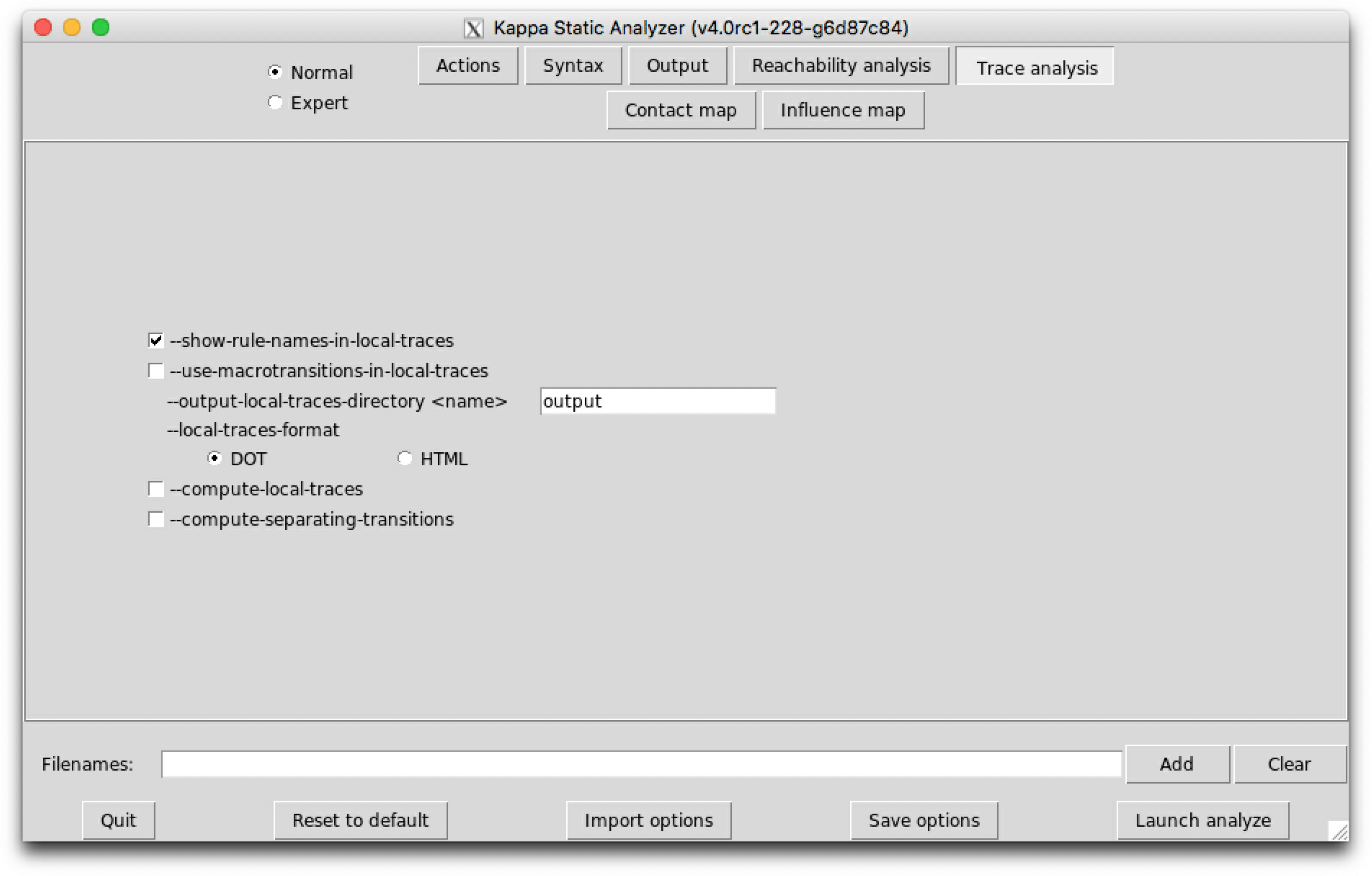
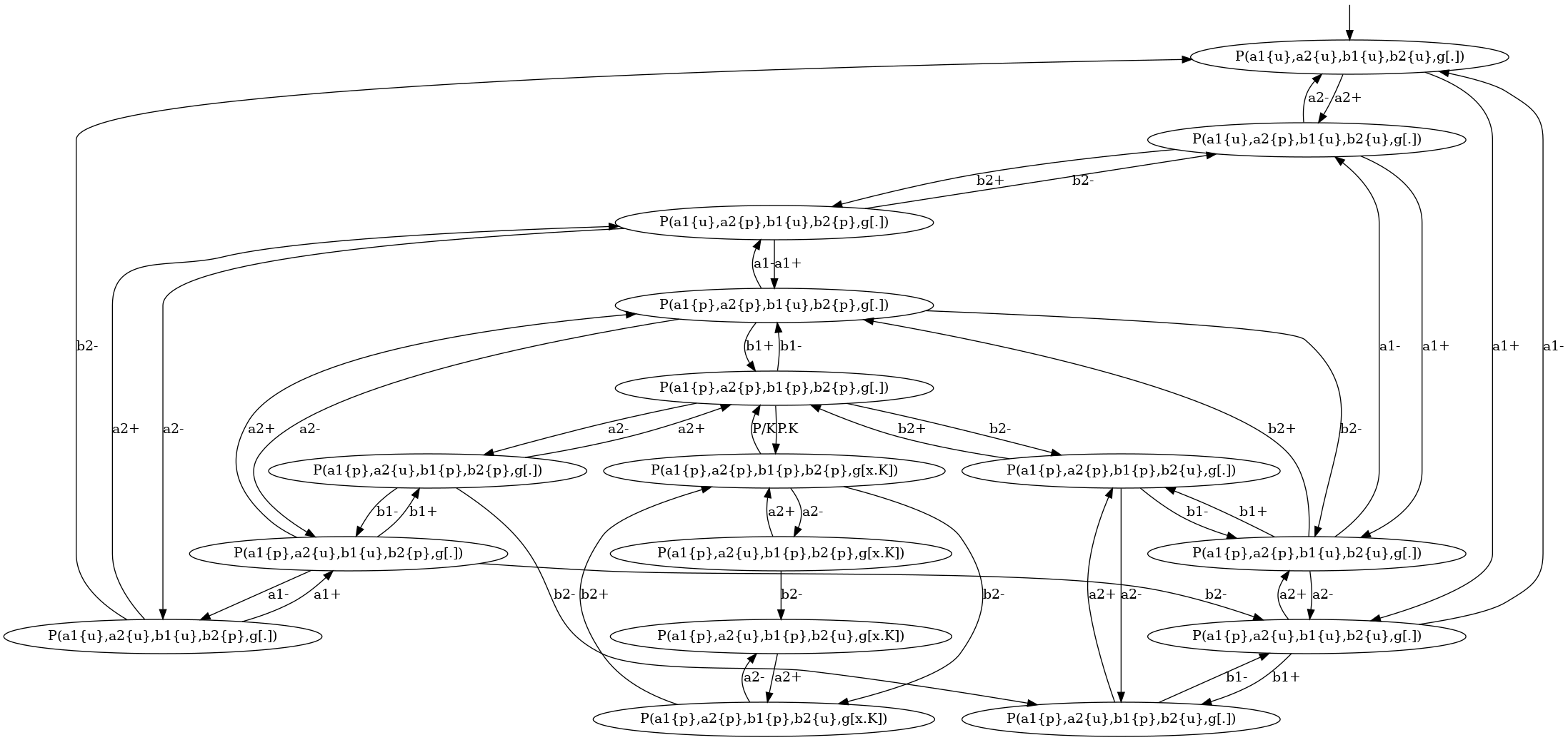
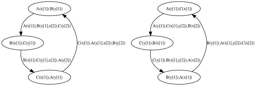
Trace analysis is a refinement of reachability analysis that additionaly explains how one agent can go from a given view to another one, following a path that we call a local trace. Thus the set of the local traces for a given agent can be described as a transition system among the views for a given agent: in this transition system, the nodes are local views; introduction arrows correspond to either initial states, or creation rules; transitions denote a potential conformation change of an agent, from one local views to another one, due to the application of a given rule.
We consider the following example:
Typing the following command line:
will perform the trace analysis on the model protein2x2.ka, and produce two dot format files Agent_trace_K_x^.dot and Agent_trace.P.a1_.a2_.b1_.b2_.g^.dot. The output repository can be changed thanks to the command line options --output-directory and --output-local-trace-directory. Moreover, file names are made of the prefix Agent_trace, followed by the kind of protein and the list of the sites of interest (the symbol ‘^’ denotes a binding state, and the symbol ‘_’ an internal state).
The transition system that describes the local traces for the agents of kind is descrided in Figure 6.14. We notice that the nodes of this transition system are labelled with the states of the sites of . The internal state of a site is denoted as (meaning that the site has state , whereas the binding state of a site is denoted as , when the site is free, and as when the site is bound to the site of a given agent of kind .
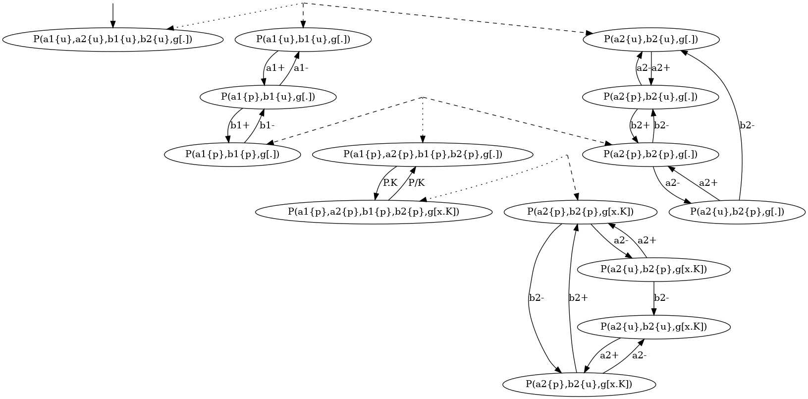
We notice that the transition system that is given in Fig. 6.14 contains too many nodes. We can coarse-grain this transition system thanks to the following option:
--use-macrotransitions-in-local-traces.
Typing the following command line:
will perform the trace analysis on the model protein2x2.ka, and produce two dot format files Agent_trace_K_x^.dot and Agent_trace.P.a1_.a2_.b1_.b2_.g^.dot. The name of the output repository can be changed thanks to the command line options --output-directory and --output-local-trace-directory. This time, the files describe a coarse-graining of the corresponding transition systems.
For instance, the coarse-grained transition system for the local traces of the proteins of kind is given in Figure 6.15. This coarse-grained transition system is a compact implicit encoding of the transition system in Figure 6.14. It is obtained by exploiting the fact that locally, the behavior of the pair of states and is independent from the behavior of the pair of states and , until these four sites are phosphorylated, so that the site can get bound.
More formally, in that transition system, some states are microstates (in a microstate, the state of each site is documented); some others are macrostates: (in a macrostate, the states of only a subset of site is documented). Thus a macrostate can be seen intensionally as a part of a local view, but also extensionnaly as the set of the local views they are a subpart of. A microstate can be described by any sequence of macrostates providing that the intersection of the extensional denotation of these macrostates is equal to the singleton ; moreover a transition between two microstates and can be described by any transition between one macro state and another one , provided that there exists a sequence of macrostate such that the sequence denotes the microstate and the sequence denotes the microstate .
Such coarse-grained transition system can be geometrically interpreted as a simplicial complex [15].
As a microstate could be decomposed into several sequences of macrostates (including the trivial sequence containing only the microstate itself), the system may jump spontaneously (by using a transition) from one representation to another representation. This corresponds to the intersection between several simplexes in the corresponding simplificial complex.
Although the semantics of a coarse-grainged transition system is fully defined by its labelled transitions, it is useful to annotate the graph by some information about the relation between the denotation of each macrostate. By default, we use hypertlinks to relate each macrostate (including each microstate) to the set of its immediate subparts . In such a hyperlink, is connected via a dotted arrow, whereas each immediate subpart is connected via a dashed arrow.
More options are available in expert mode, but they are not documented yet.
The contact map of a model is an object that may help modelers checking the consistency of the rule set they use. The contact map is statically computed and does not depend on kinetic rates, nor the concentration of the bio-molecular species in initial state.
Typing the following command line:
KaSa abc.ka –reset-all –compute-contact-map
will produce a dot format file named contact.dot. The name of the output file and the directory can be changed thanks to the command line options --output-contact-map and --output-directory. The directory is assumed to exist. The file will be overwritten if it exists. All the options related to the computation of the contact map can be accessed on the sub-tab Contact map of the graphical interface (see Fig. 6.16).
The contact map summarises the different types of agent, their interface and the potential bindings between sites. It is an over approximation, thus if the contact map indicates a potential bond, it does not mean that it is always possible to reach a state in which two sites of these kinds are bound, but if the contact map indicates no bond between two sites, it means that it is NOT possible to reach a state in which two sites of these kinds are bound together.
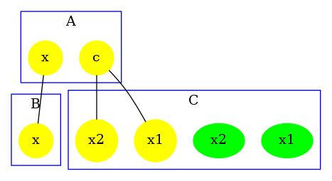
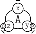
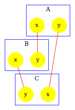
The contact map for the abc.ka model defined in Chapter 1.3 is given in Figure 6.17. On this map, we notice that there are three kinds of agent, namely , , and . Agents of kind have two sites and , that bear no internal state (they appear in yellow only), agents of kind have one site , that bears no internal state (they appear in yellow only), and agents of kind have two sites and with both a binding state and an internal state (they appear both in yellow and in green). We notice that when a site can bear both an internal state and a binding state, they are considered as two different sites in the contact map. Additionally, the contact map indicates that sites of the agents of kind can be bound to the site of an agent of kind and that sites of the agents of kind can be bound to the agents of kind either on the site , or on the site .
There exist two accuracy levels for the contact map. At low level of accuracy, the inference of the contact map is purely syntactic. The contact map summarizes the bonds that may occur in the right hand side of rules and in the initial bio-molecular species. At high level of accuracy, the rules that are detected dead by the reachability analysis are not taken into account. Hence, only the bonds that may occur in the initial bio-molecular species, and in the rules that have not been proven dead by the static analysis are reported. As a matter of fact, the accuracy of the computation of the contact map at high level of resolution depends on the parameterization of the reachability analysis.
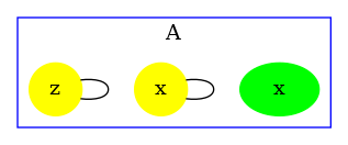
Let us illustrate this on a simple example. The file contact.ka has the following content:
Firstly we compute the low resolution contact map by using the following instruction:
We obtain the contact map that is drawed in Fig. 6.18. We notice that the analysis reports a potential bond between the sites of any two agents of type and a potential bond between the sites of any two agents of type . This is because such bonds occur in the right hand side of some rules of the model.
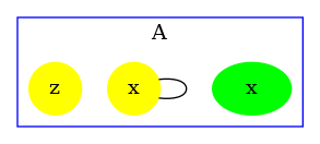
Yet, bonds between two sites occur only in the last rule which turns out to be dead. Let us use the high resolution contact map to check this property. We use the following instruction:
We obtain the contact map that is drawed in Fig. 6.19. We notice that the potential bond between sites of agents has disappeared: the result of the analysis has been refined thanks to the constraints infered by the reachability analysis.
The proof that, the last rule of the model in the file contact.ka is dead relies on the abstract domain, that captures the potential relationships between states of sites in the pairs of agents, that are connected by a bond. Let us compute the high resolution contact map without this abstract domain:
We obtain the contact map that is given in Fig. 6.20. The analysis has failed in proving that the last rule of the model is dead. As a matter of fact, the potential bond between sites of agents has not disappeared.

The contact map may be refined with information about polymers. When the commmand line option –compute-potential-cycles is used, KaSa computes a superset of the bonds the number of occurences of which may not be uniformly bounded in paths within bio-molecular species. These bonds are then displayed in red in the contact map.
The computation of this subset is based on Tarjan’s algorithm for the decomposition of a graph in strongly connected components [25]. For this, we consider the graph of the potential succesion of bonds in bio-molecular species. The nodes of this graph are the oriented version of the potential bonds in the contact map (each potential bond is considered twice). Then there is an edge between two oriented bonds if the target of the first bond and the source of the second bond have the same agent type but different site names. Hence each edge is associated with a graph that is obtained by merging the graph associated to the source and the target of this edge, that is to say that each edge is associated with a graph made of three agents and two bonds (e.g. see Fig. 6.21). We can notice that every path that may be repeated in bio-molecular species necessarily forms a cycle in this graph. The computation of all the elementary cycles in graph may be exponentially costly. Instead, we compute the strongly connected components which can be done in linear time (with respect to the sum among the number of nodes and the number of edges in the graph). The computation of the strongly connected components is enough, since an edge belongs to a cycle if and only if it belongs to a non trivial strongly connected component.
The file scc_abc.ka has the following content:
In this example, arbitrary long chains and arbitrary long rings of agents may be formed (the site of each is either free or bound to the site of a ; the site of each is either free or bound to the site of a ; and the site of each is either free or bound to the site of a ).
The graph that is associated to this model is given in Fig. 6.21.
Typing the following command line:
will generate the contact map that is given Fig. 6.22
The accuracy of the detection of polymers may be tuned in two ways. Firstly, it is parameterized of the accuracy of the contact map. Secondly, it may be refined by the reachability analysis in order to discard the couple of bonds that cannot be present successively in reachable bio-molecular compounds.
The file scc_relations.ka contains the following model:
In this model, the sites and of a given instance of the agent cannot be bound simultaneously. This prevents the formation of polymers.
By default, the detection of polymers is using the result of the reachability analysis. Thus, the following instruction:
produces the contact map that is drawed in Fig. 6.23. By default, the detection of polymers has used the result of the reachability analysis: since the bonds on the site and of each instance of the agent are mutually exclusive, no polymer may be formed.
The refinement by the result of the reachability analysis can be disable by using the following instruction:
In this case, KaSa produces the contact map that is given in Fig. 6.24. The analysis does know that the bonds of the sites of each agent of type are mutually exclusive. The bonds are drawed in red to warn about the potential formation of polymers of the model (this is a false alarm).
The detection of polymer at high resolution also depends on the accuracy of the reachability analysis. The file scc_dimer.ka contains the following model:
In this model, two agents of type may connect their sites together. Then, two agents connected via their sites may establish an asymetric bond between the site of the first one and the site of the second one. As a consequence, whenever an agent of type has several sites bound, these sites are necessarily bound to the same instance of the agent . Thus, there can be no polymer.
At low resolution, the detection of polymer fails in exploiting this property, and warns about potential polymers. Indeed, the following instruction:
produces the contact map that is drawed in Fig. 6.25.

At high level of resolution, the analysis for the detection of potential polymers successfully prove the lack of polymers. The following instruction:
produces the contact map that is given in Fig. 6.26. The analysis has successfully proven the lack of polymers (no bond is colored in red).
In order to illustrate that the accuracy of the analysis relies in this example on the capability for the analysis to exploit properties of double bonds. We disable the double bond domain. The following instruction:
produces the contact map that is given in Fig. 6.27. Without the capability to express and prove that whenever an agent of type is bound twice, it is necessarily bound twice to the same agent instance. The analysis fails in proving the absence of polymer. Thus, it warns about potential polymers, by drawing the edges in red.
The influence map of a model is an object that may help modelers checking the consistency of the rule set they use.
Typing the following command line:
KaSa abc.ka –reset-all –compute-influence-map
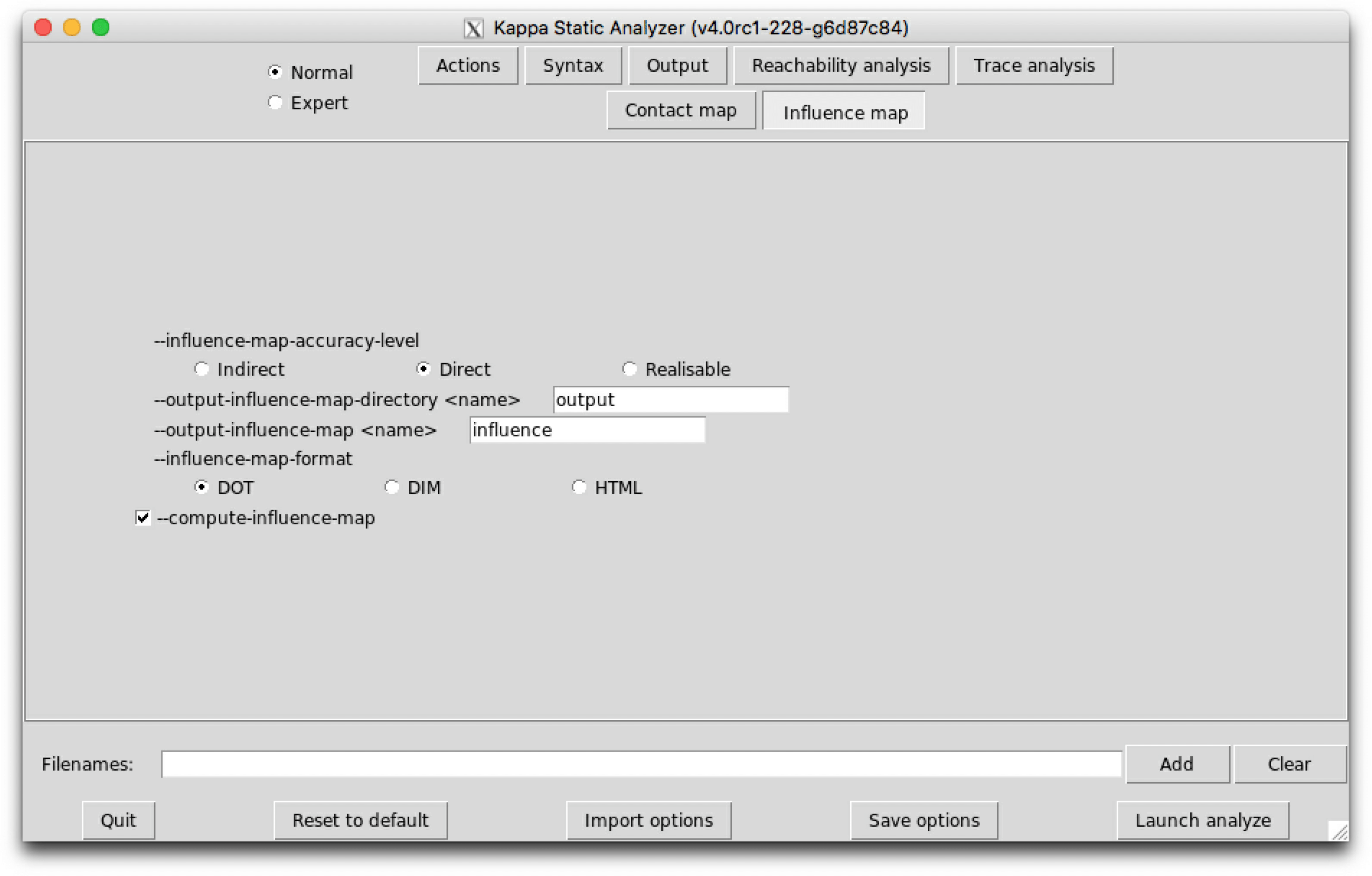
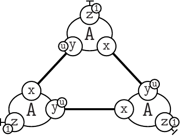
will produce a dot format file named influence.dot. The name of the output file and the directory can be changed thanks to the command line options --output-influence-map and --output-directory. The directory is assumed to exist. The file will be overwritten if it exists. All the options related to the computation of the influence map can be accessed on the sub-tab Influence map of the graphical interface (see Fig. 6.28). Two formats are available for the output: influence map can be generated in DOT or HTML format. The format can be choosen thanks to the command line option --influence-map-format.
Unlike the dynamic influence network, the influence map is statically computed and does not depend on kinetic rates nor the quantities in initial conditions. It describes how rules may potentially influence each other during a simulation. KaSa will produce a dot format file containing the influence relation over all rules and observables of the model. The produced graph visualised using a circular rendering1 is given in Figure 6.29. Observables are represented as circular nodes and rules as rectangular nodes. The labels of the nodes are either the label of the rule or of the observable (if available), otherwise they are made of a unique identifier allocated by KaSa followed by the Kappa definition of the rule/observable. Edges are decorated with the list of embeddings (separated by a semi-colon) allowing the identification of agents in both rules’ right hand sides/left hand sides. More precisely, for positive influences, the notation denotes a pair of embeddings from the agent number of the origin's right hand side and from the agent number of the target's left hand side and the notation denotes a pair of embeddings from an agent attached to the agent number of the origin's left hand side, which have been freed by side effect and from the agent number of the target's left hand side; for negative influences, the notation denotes a pair of embeddings from the agent number of the origin's left hand side and from the agent number of the target's left hand side and the notation denotes a pair of embeddings from an agent attached to the agent number of the origin's left hand side, which have been freed by side effect and from the agent number of the target's left hand side; Observables have no influence, but they can be influenced by rules, if the rule can increase or decrease their value.
More formally, consider the rules and . One wishes to know whether it is possible that the application of rule over a graph creates a new instance of rule (which is called a positive influence and that is described by green arrows in the influence map), or destroy a previous instance of rule (which is called negative influence and that is described by red arrows in the influence map). In Fig. 6.30, we illustrate the construction of positive influences due to overlap of the left hand side of a rule and the right hand side of another rule on some sites that are modified by the former one.
The current implementation has the following limitations:
Lastly, KaSa computes an over-approximation of the influence map. They may show an influence despite the fact that there can be no actual one. But if it shows no influence it means that either there are NO such influence, or that we are in a case that is not covered yet as itemised previously.
Three levels of precision are available: Low, Medium, and High. The level of precision can be changed thanks to the command line option --influence-map-accuracy-level.
At low precision, an influence is detected if one rule change at least one bit of information (the internal state of a site, the binding state of a site), in favor/defavor of the application of another rule. This abstraction level ignores completely the context of application of rules, and just focuses on modifications.
At medium precision, the analysis checks that both rules have a common context.
At high precision, the analysis checks that such common context is realizable taking into account the species that have been declared as initial states and the potential introduction of species in interventions. High resolution influence is parameterized by the accuracy of the reachability analysis. It may happen that a given context is infeasible, but that this is not detected by the analysis.
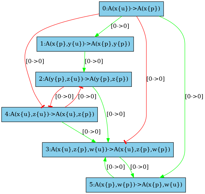
Let us illustrate these three levels of accuracy by a case study.
We consider the following model.
The low resolution influence map is given in Fig. 6.31. There is a positive arc (in green) from a rule to another one whenever the application of the former pushes at least one bit of information towards the application of the later; whereas there is a negative arc (in red) from a rule to another one whenever the former pulls at least one bit of information away from the application of the later.
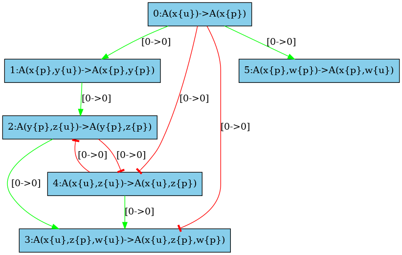
The medium resolution influence map is given in Fig. 6.32. Every arc corresponding to incompatible contexts has been removed. In our example, these are the arcs from the rule and the rule (in both direction). Despite the fact that the rule may phosphorylate the site w which is required to apply the rule , no instance of the rule may be applied thanks to the application of the rule right after, because after the application of the rule the state of the site is necessarily unphosphorylated, whereas it has to be phosphorylated for the rule to be applied. The same kind of explanation holds to remove the arc from the rule to the rule .
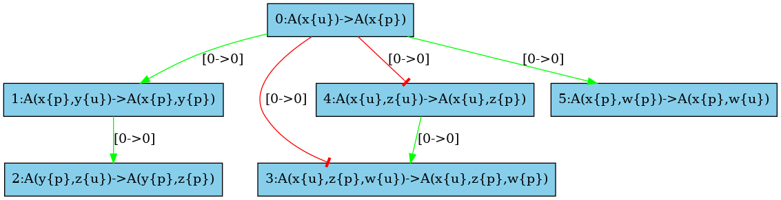
There are some structural invariants in these models. We give in Fig. 6.34 the log of the computation of the high resolution contact map. It turns out that whenever the site y of an agent is phosphorylated, then the site x of this protein is phosphorylated as well. Thus we can deduce that the positive arc from the rules and , and the negative arcs from the rules and (in both direction) are false positive unless we change the set of the species in the initial state or in the interventions. Thus we obtain the high resolution influence map given in Fig. 6.33.
From a terminal window, KaDE can be invoked by typing the following command line:
where file_i are the input Kappa files containing the rules, initial conditions and observables (see Chapter 2).
All the options are summarised as follows:
Orders in option matter, since they can be used to toggle on/off some functionalities or to assign a value to some environment variables. The options are interpreted from left to right.
The graphical interface can be launched by typing the following command line:
without any option.
There are five different areas of importance in the graphical interface:
Contextual help is provided when the mouse is hovered over an element. The interface will store the options that are checked or filled and the order in which they have been selected. When launched, the analysis interprets these options in the order they have been entered. Some options appear in several sub-tabs. They denote the same option and share the same value.
Importantly, options are saved automatically under various occasions. Thus, it is possible to restore the value of the options before the last reset, before the last quit, or before the last analysis.
Two fields define the repository and the name of the output:
Both fields may be modified from every sub-tab.
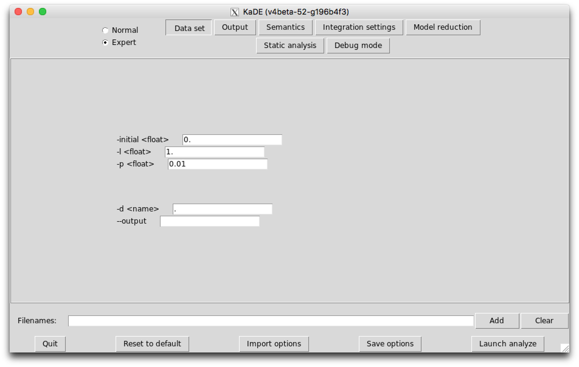
The sub-tab Data set (see Fig. 7.1) contains the options to tune the time range for the numerical integration and the frequency of sample plots. These fields are used only in Maple, Mathematica, Matlab, and Octave backend formats. They are ignored in SBML and DOTNET backend formats.
The following options are available:
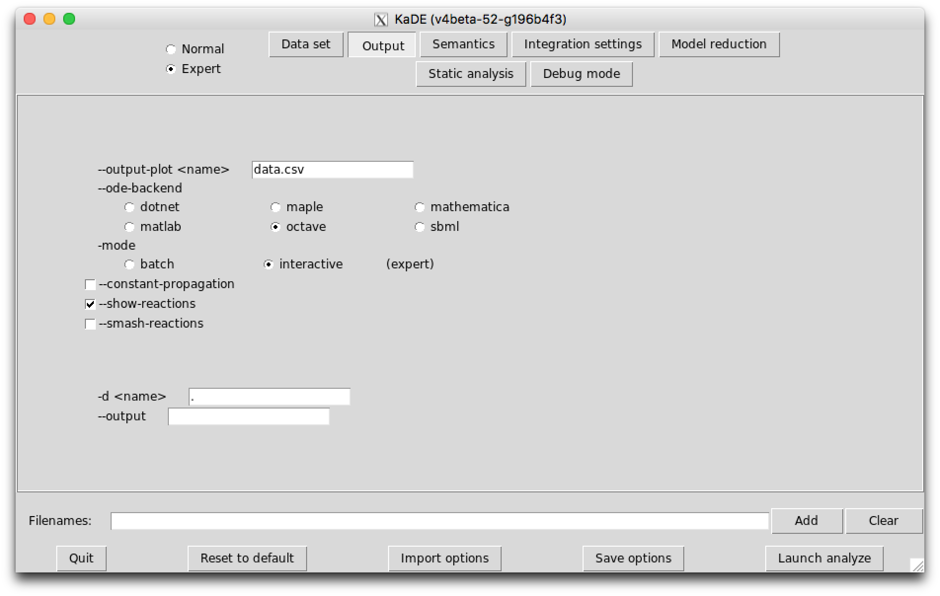
The sub-tab Output (see Fig. 7.2) contains the names of the output files and their format.
The following options are available:
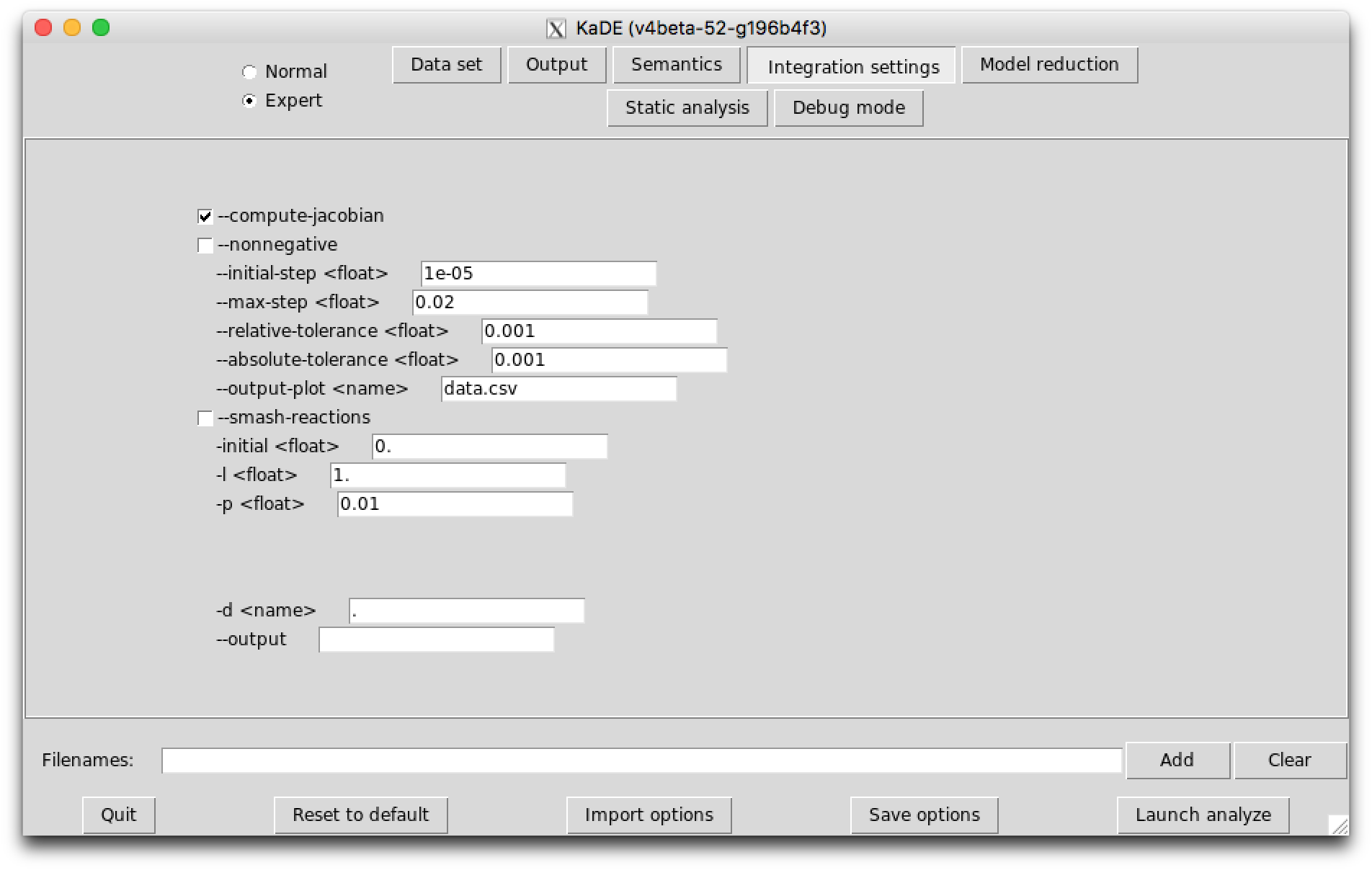
The sub-tab Integration settings (see Fig. 7.3) contains the parameters to guide the numerical integration engine. Except the option --smash-reaction, these options are ignored in the SBML and the DOTNET backend format.
The following options are available:
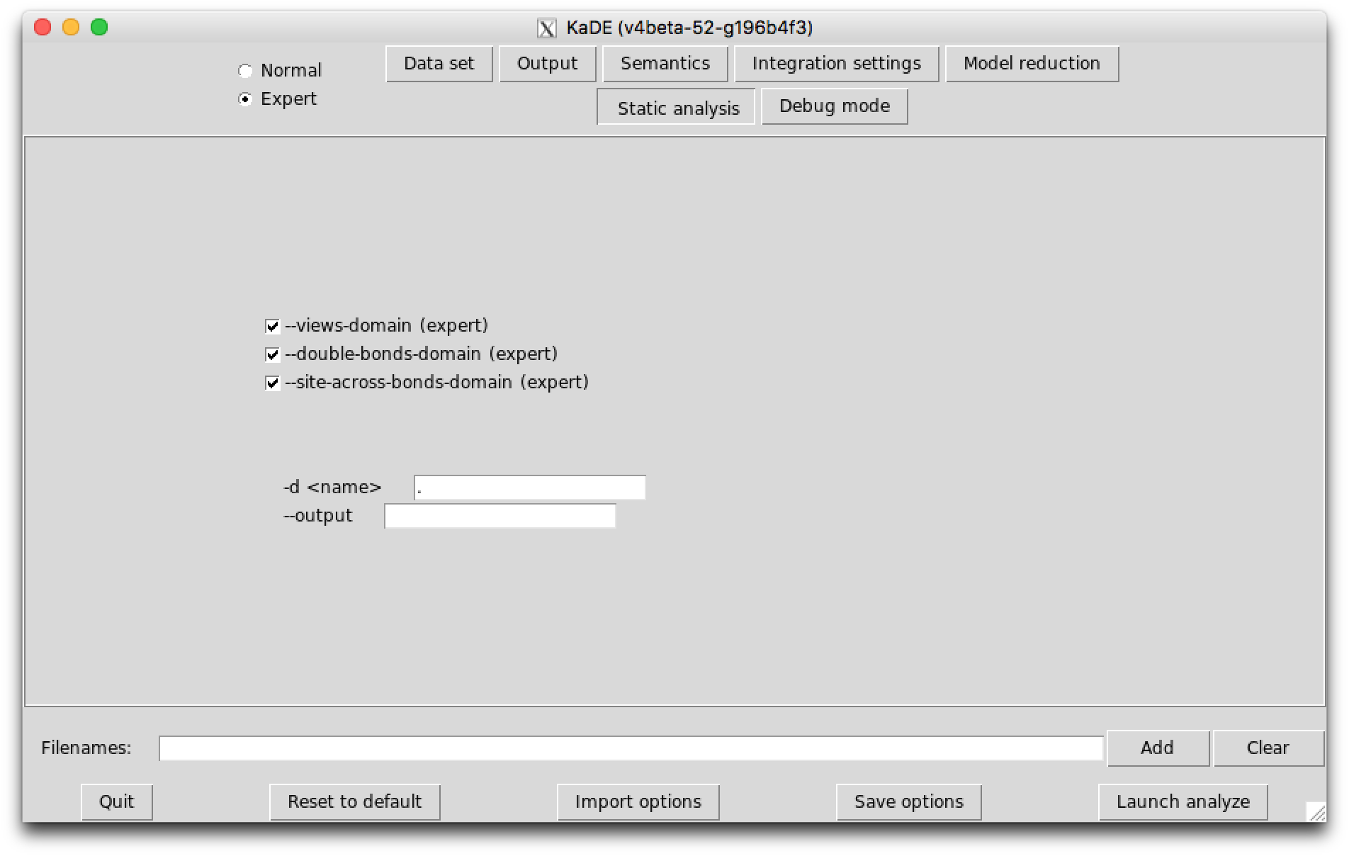
In expert mode, the last sub-tab provides options to tune the amount of debugging information that is displayed.
The following options are available:
In Kappa, rules may be more and less refined [7, 9], according to their preconditions.
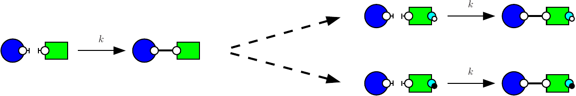
Consider the following two rules:
The first rule (e.g. see Fig. 7.5) stipulates that proteins of type K and proteins of type S may bind via their respective right and left sites. The second rule (e.g. see Fig. 7.6) stipulates that a protein S bound to a protein K may be activated (on its right site).
It is worth noticing that the first rule may be applied in two different contexts, according to whether or not the right site of the protein on the right is already phosphorylated, or not. It follows the refinement that is depicted in Fig. 7.7.
In general, each rule may be refined into a (potentially infinite) multi-set of reactions over fully specified site-graphs. Each connected component in a reaction denotes an instance of a bio-molecular species. For every bio-molecular species , a reaction gives the following contribution to the derivative of the concentration of ,
where:
This defines the ODE semantics of Kappa models.
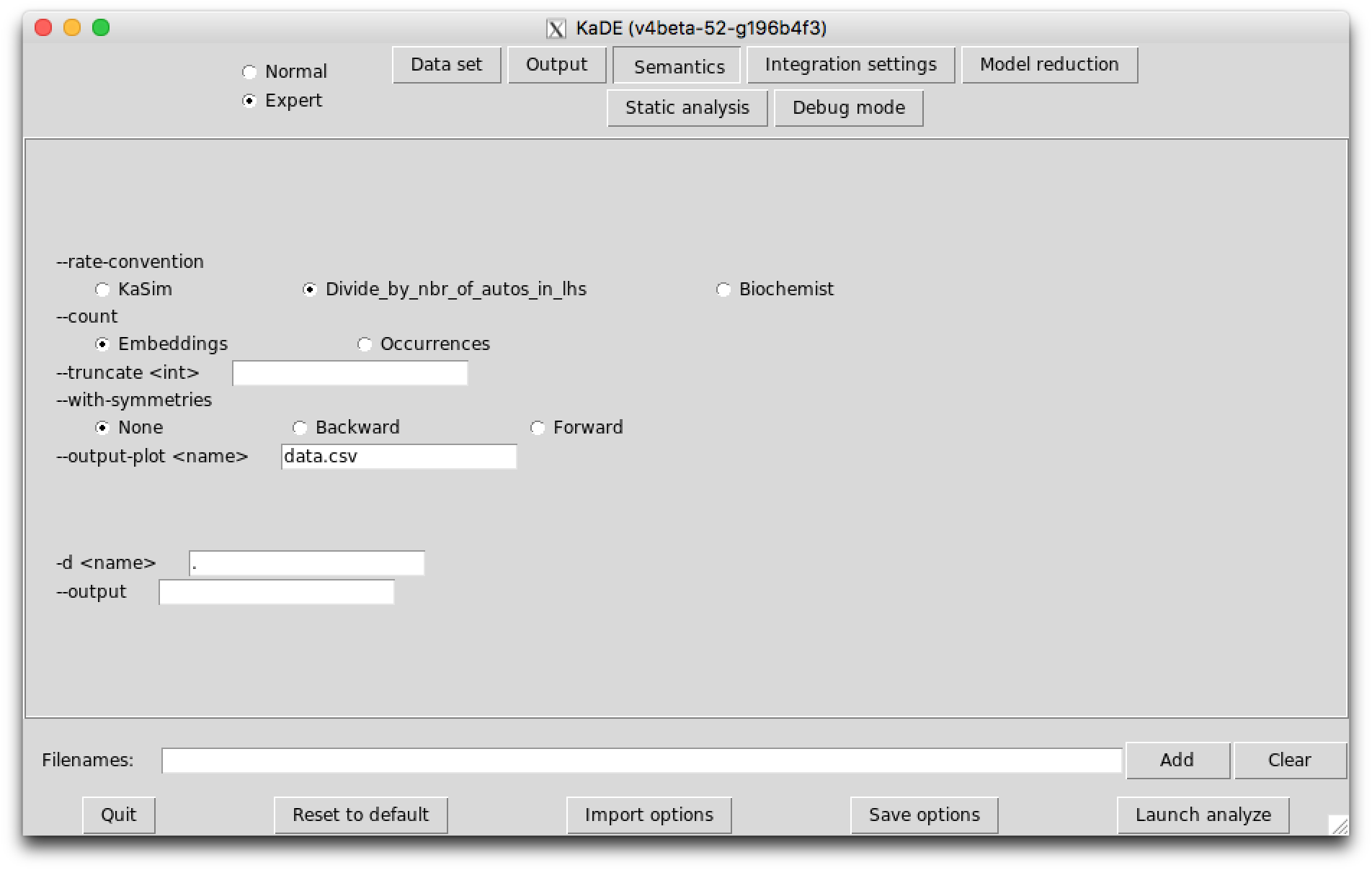
The options in the sub-tab Semantics allow for the choice among several possibilities for the meaning of the ODEs variables and for the meaning of the rate constants.
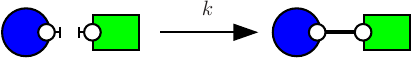
KaDE corrects the rate constant of each according to a convention about the number of automorphisms in this rule. KaDE offers the choice among three conventions:
Consider the following rule:
which is depicted as follows:

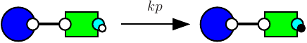
with the first convention (that is the one of the simulator), rates of rules are not corrected, hence the effective rate of this rule is ; with the second one, rates are divided by the number of automorphisms in the left hand side of rules (here that is to say ); the third convention accounts only for the permutations among the agents that are undistinguishable from a mechanistic point of view: rates are divided by the number of automorphisms in the left hand side of rules that also induce automorphisms of the right hand side (here ).
The differential semantics is defined as the limit of the stochastic semantics when the temperature diverges toward the infinity. Thus a rate constant stands indeed for a function mapping the temperature to an effective rate constant the expression of which depends on the arity of the reaction. Even if the unary rate and the binary rate of a rule may be equal for a given temperature, it is never the case at all temperatures. Another insight is that rate constants for a unary reaction and rate constants for a binary reaction are not expressed in the same physical units.
To account for this, KaDE never applies a binary rule in a unary context, unless two rate constants have been provided explicitly.
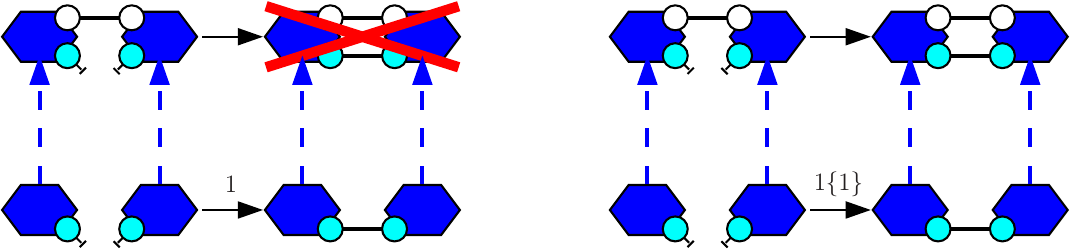
Let us give an example. We consider the agent type A with two binding sites x and y. We assume that two sites x (in different As) may be bound pair-wise and that two sites y (in different As) may be bound pair-wise. Both following rules:
will behave the same: they both apply to the following mixture
but not to the following one:
So as to allow the rule to form a bond within the two agents of the dimer, the following rule:
shall be used instead.
This way, when a rule is given with one rate constant only, the connected components in its left hand side have to be refined into pair-wisely disjoint bio-molecular species. When a rule is binary and when it is given with two rate constants, it may be apply in a unary context (which consists in embedding its left hand side into a single bio-molecular species) with the second rate constant, or in a binary context (which consists in embedding each connected component in its left hand side into two disjoint bio-molecular species (which may be two isomorphic copies of the same species)).
In a Kappa file, a pattern may denote two different quantities. At initialisation, a pattern denotes an occurence of a bio-molecular species. In an algebraic expression (which includes functional rates, stoichiometric coefficients for tokens, observables), a pattern denotes a number of embeddings from this pattern to a mixture.
Formally, we define the number (resp. the concentration) of embeddings from a pattern to a mixture (resp. to a concentration function) as the sum, for each bio-molecular species, of the number of occurrences (resp. concentration) of that bio-molecular species and the number of occurrences of the pattern in that bio-molecular species. We also define the number (resp. the concentration) of occurrences of a pattern in a mixture (resp. in a concentration function) as the quotient between the number (resp. the concentration) of embeddings from this pattern to a mixture (resp. to a concentration function) and the number of automorphisms in this pattern.
To illustrate this, we assume that the file occ.ka contains the following code:
We use the following command line to get the value of the observable:
The file csv contains the following data set:
We notice that KaSim indicates for the quantities of dimers. This accounts for the fact that each dimer satisfies two automorphisms.
The command-line option --count [Embeddings | Occurrences] changes the meaning of the variables that occur in the differential equations. The choice has no impact on the quantities that are plot. Introduced bio-molecular species are always introduced in concentration of occurrences, and patterns in algebraic expressions always denote concentration of embeddings. It just changes the meaning of the variables that are used internally in the differential equations.
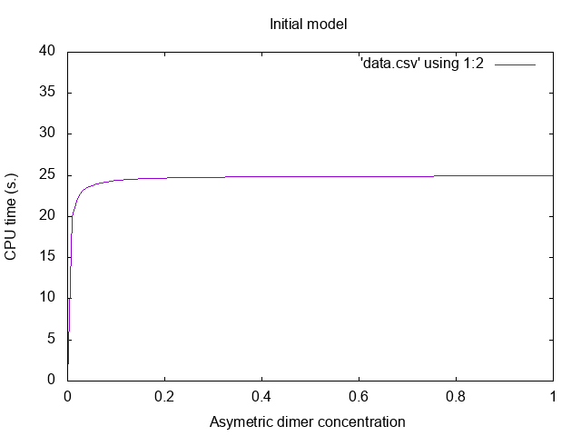
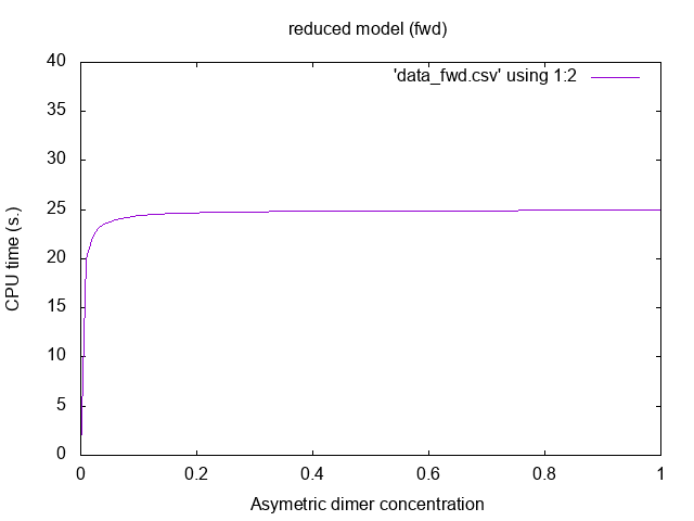
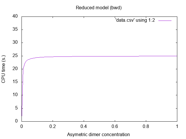
In case of polymerisation, the size of the bio-molecular species is potentially unbounded and there may be an infinite amount of differential equations (this is the case even if there is no agent synthesis, since the initial state is given in concentration, and not in occurrence number). In such a case, KaDE will not terminate. Yet it is possible to truncate the system of ordinary differential equations: the command-line option --truncate specifies an upper bound to the number of agents in the bio-molecular species. Each reaction that would involve a larger bio-molecular species is discarded.
For instance, we can consider the model poly.ka that is defined as follows:
The command line:
will not terminate, wheareas the following one:
will.
In BNGL, the interface of a given agent may include several occurrence of a given site name. These sites have exactly the same capabilities of interaction. This feature provides a convenient syntactic construction to describe models even more compactly, at the cost of having to deal with more complex structures (detecting embeddings between such site-graphs may be very difficult).
In Kappa, the interface of every agent is made of pair-wisely distinct site names. Yet it may happen that some sites have exactly the same capabilities of interaction. KaDE can infer this property and use it to derive a more compact system of differential equations [3, 4, 18].
Consider the following model:
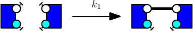
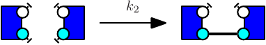
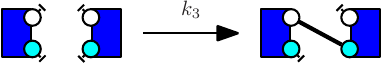
The rules are depicted in Fig. 7.10. We notice that each rule may be obtained from one another by swapping the sites in agents. So we say that sites are equivalent in this set of rules. Equivalent sites may be used to induce forward and backward bisimulations [2, 19, 3, 4, 18] over the stochastic and the differential semantics of Kappa.
Let us consider two site names x and y in the signature of an agent type A. A set of rules is symmetric with respect to x and y, if for every two rules that may be obtained one from the other one by permuting the sites x and y in some agents of type A, their corrected rates is inversely proportional to their number of automorphisms. In our example, the set of rules is symmetric with respect to x and y only with the convention in which constant rates are kept as they are given, without any corrective factor. A valuation from bio-molecular species to real numbers is symmetric with respect to x and y, if for every two bio-molecular species that can be obtained one from the other one by permuting the sites x and y in some agents of type A, the image of the two bio-molecular species by the valuation is inversely proportional to their number of automorphisms. Lastly an expression over bio-molecular species is symmetric with respect to x and y, if and only if it takes the same values for every two symmetric valuations.
If the set of rules and the initial state of the model are symmetric with respect to two sites, ignoring the difference among these two sites in bio-molecular species induces a backward bisimulation (that is to say, the state of the system remains symmetric at every time [1]). If the set of rules and every algebraic expression that occurs in rates or stoichiometric coefficients are symmetric, then ignoring the difference between these two sites in bio-molecular species induces a forward bisimulation (we can define the ODEs directly over the equivalence-classes of bio-molecular species [1]).
The following option is available:
The sub-tab Model reduction gives access to more information about potential model reduction.
The following options are available:
The inference of equivalent sites is more precise when dead rules are discarded. Dead rules can be computed thanks to KaSa. The sub-tab Static analysis allows the end-user to switch on/switch off abstract domains in order to tune the trade-off between accuracy and efficiency of static analysis.
The following options are available:
Now we explain further how to use KaDE to deal with the example of Sect. 7.3.2. The model is described in the following Kappa file:
The rules of this models are depicted as follows:
We denote as , , and the corrected rate constants of these rules. With the third convention, which roughly speaking consists in dividing rates per the number of automorphisms in the left hand side of rules, that are preserved in the right hand side, we have:
Indeed, in the third rule, the mechanism makes a difference among the two agents. The non trivial automorphism in the left hand side is not preserved in the right hand side.
Rules and have two automorphisms, whereas rule has only one. As a consequence, the rules are symmetric with respect to both sites if and only , that is to say .
We use the following command line to generate the ODE semantics in Octave:
By default, equivalent sites are not analysed and the Octave backend is used.
The result is dumped in the file ’ode.m’, which is editable. Moreover, each instruction is annotated with some information referring to the Kappa file. Variables are annotated by the corresponding name in the Kappa file. Initial species are annotated by Kappa expressions describing the corresponding bio-molecular species.
Integration parameters are defined as follows:
The variable nodevar gives the number of variables:
The function ode_init defines the list of variables and their initial concentration:
We notice that four variables encode the concentration of bio-molecular species and a special one accounts for time advance.
The function dydt defines the differential equations:
The function obs defines the observables:
The function jac provides the Jacobian (we omit it).
We now wonder whether the sites are equivalent or not. We use the following command line:
The status of equivalent sites is described in the log:
The set of rules and the initial state are symmetric with respect to the pair of sites. This is not the case of the observable. Thus, only backward bisimulation may be used to reduce the system. Indeed, if we ignore the difference between sites x and y, we can no longer express the concentration of asymmetric dimers. This excludes forward bisimulation. Backward bisimulations may still be used since the concentration of each species can be computed by from the overall concentration of its equivalence class, since the concentration of two equivalent species are always inversely proportional to their number of automorphisms.
The command line:
gives the same model, without any reduction.
The command line:
reduces the system by ignoring the difference between sites x and y. This is done by replacing in each reaction product, every species by an arbitrary representative of its equivalence class, and in each algebraic expression, each species concentration by the product of its the concentration of its representative times the relative weight of this species in its equivalence class (which is constant and inversely proportional to its number of automorphisms.)
We notice that there are only variables remaining:
one for time advance, one for free As, and one for dimers (no matter which sites are bound). KaDE has gathered the three kinds of dimers into a single equivalence class (no matter with sites are bound). For instance, in the following:
the production of an asymmetric dimer, is replaced with the production of a dimer in which the bond is on both sites y.
Now we explain how the values of the obervavles are computed. The code for the function obs is the following one:
We are interested in asymmetric dimers only. We notice that their concentration is obtained by dividing the overall quantity of dimers by . To understand why, we shall have a closer look at the meaning of each variable. As indicated here:
the convention is to count in number of embeddings. Thus the total number of dimers is . Then half of them only is an asymmetric dimer, which gives .
Let us check the soundness of our tools, by integrating our three ODEs systems.
Firsly we define the file plot.gplot as follows:
the file plot_fwd.gplot as follows:
and the file plot_bwd.gplot as follows:
Then we can integrate our three differential systems and plot their respective solutions thanks to the following command lines:
We obtain the following plots:
If the progress bar seems stalled, it does not necessarily mean that the simulation is blocked. In particular when a simulation is triggered with a time limit (-l option of the command line) it might only indicate that the bio clock is stalled while computation events still occur. Recall that the average (bio) time one has to wait in order to apply a rule is , where is the sum of all the rule activities (which is equal to the number of instances that a rule has, times its kinetic rate). Whenever the number of occurrences of a rule grows too fast (if new agents are created during the simulation for instance), or if the kinetic rate of a rule is defined by a function that grows rapidly, the average time increment might tend to 0 and if it remains so for a while, it will block the progress bar whose advance is proportional to the bio time [T].
In order to make sure that KaSim is not incorrectly blocked you may wish to plot the event clock against time clock using the observable %obs: 'events' [E] or run the simulation using an event limit (-e option of the command line) instead of a time limit.
Using null events is a way for KaSim to compensate for some over approximation it is doing, in order to deal with large simulations more efficiently. They usually do not impact significantly the performances of the simulator, unless the model contains rules using the special notation to deal with ambiguous molecularity (see Section 2.5.4). With pure Kappa rules, the ratio of null event over productive ones (that you can track using the observable %obs: 'r' [E-]/[E]) should tend to 0 when models have a lot of agents.
Make sure you have %obs or %plot instructions in your KF. Also make sure to use a reasonable value for the -p option in the command line to tell KaSim how often you wish to have points on your curves.
The value of a Kappa expression is equal to the number of embeddings it has in the current mixture . Embeddings are maps from agents in to agents in . If has symmetries then every permutation of will be counted as a new embedding. For instance let A(x[1]),A(x[1]) and let A(x[1],y{p}[.]),A(x[1],y{u}[.]). KaSim will count two instances of in : the one mapping the first A of to the first A of and the one mapping the first A of to the second A of .
The value nan means "Not a Number". It is generated when a plotted variable is infinite. Make sure this variable is not divided by zero at some point.
[1] Peter Buchholz. Exact and ordinary lumpability in finite Markov chains. Journal of Applied Probability, 31(1):59–75, 1994.
[2] Peter Buchholz. Bisimulation relations for weighted automata. Theoretical Computer Science, 393(1-3):109–123, 2008.
[3] Ferdinanda Camporesi and Jérôme Feret. Formal reduction for rule-based models. In Postproceedings of the Twenty-seventh Conference on the Mathematical Foundations of Programming Semantics, MFPS XXVII, volume 276C of Electonic Notes in Theoretical Computer Science, pages 31–61, Pittsburg, USA, 25–28 May 2011. Elsevier Science Publishers.
[4] Ferdinanda Camporesi, JÃľrÃťme Feret, Heinz Koeppl, and Tatjana Petrov. Combining model reductions. Electronic Notes in Theoretical Computer Science, 265:73 – 96, 2010.
[5] P. Cousot and R. Cousot. Static determination of dynamic properties of programs. In Proceedings of the Second International Symposium on Programming, pages 106–130. Dunod, Paris, France, 1976.
[6] Patrick Cousot, Radhia Cousot, Jérôme Feret, Laurent Mauborgne, Antoine Miné, David Monniaux, and Xavier Rival. Combination of abstractions in the Astrée static analyzer. In M. Okada and I. Satoh, editors, Eleventh Annual Asian Computing Science Conference (ASIAN’06), pages 1–24, Tokyo, Japan, LNCS 4435, December 6–8 2007. Springer, Berlin.
[7] Vincent Danos, Jérôme Féret, Walter Fontana, and Russell Harmer. Rule based modelling , symmetries, refinements. In Proc. FMSB, volume 5054 of LNCS, 2008.
[8] Vincent Danos, Jérôme Feret, Walter Fontana, Russell Harmer, Jonathan Hayman, Jean Krivine, Chris Thompson-Walsh, and Glynn Winskel. Graphs, rewriting and pathway reconstruction for rule-based models. In Schloss Dagstuhl Leibniz-Zentrum fuer Informatik, editor, FSTTCS 2012 - IARCS Annual Conference on Foundations of Software Technology and Theoretical Computer Science, volume 18 of LIPIcs, pages 276–288, 2012.
[9] Vincent Danos, Jérôme Feret, Walter Fontana, Russell Harmer, and Jean Krivine. Rule-based modelling and model perturbation. Trans. Computational Systems Biology, 11:116–137, 2009.
[10] Vincent Danos, Jérôme Feret, Walter Fontana, and Jean Krivine. Scalable simulation of cellular signaling networks. In Proc. APLAS’07, volume 4807 of LNCS, pages 139–157, 2007.
[11] Vincent Danos, Jérôme Feret, Walter Fontana, and Jean Krivine. Abstract interpretation of cellular signalling networks. In Francesco Logozzo, Doron A. Peled, and Lenore D. Zuck, editors, Proceedings of the Ninth International Conference on Verification, Model Checking and Abstract Interpretation, VMCAI’2008, volume 4905 of Lecture Notes in Computer Science, pages 83–97, San Francisco, USA, 7–9 January 2008. Springer, Berlin, Germany.
[12] Vincent Danos, Jérôme Feret, Walter Fontanta, Russ Harmer, and Jean Krivine. Rule based modeling of biological signaling. In Luís Caires and Vasco Thudichum Vasconcelos, editors, Proceedings of CONCUR 2007, volume 4703 of LNCS, pages 17–41. Springer, 2007.
[13] Vincent Danos and Cosimo Laneve. Formal molecular biology. Theoretical Computer Science, 325, 2004.
[14] James R. Faeder, Mickael L. Blinov, and William S. Hlavacek. Rule based modeling of biochemical networks. Complexity, pages 22–41, 2005.
[15] Lisbeth Fajstrup, Eric Goubault, and Martin Raußen. Detecting deadlocks in concurrent systems. In Proc. CONCUR ’98, volume 1466 of LNCS, 1998.
[16] Jérôme Feret. Occurrence counting analysis for the pi-calculus. Electronic Notes in Theoretical Computer Science, 39.(2), 2001. Workshop on GEometry and Topology in COncurrency theory, PennState, USA, August 21, 2000.
[17] Jérôme Feret. Reachability analysis of biological signalling pathways by abstract interpretation. In T.E. Simos, editor, Proceedings of the International Conference of Computational Methods in Sciences and Engineering, ICCMSE’2007, Corfu, Greece, number 963.(2) in American Institute of Physics Conference Proceedings, pages 619–622, Corfu, Greece, 25–30 September 2007. American Institute of Physics.
[18] Jerome Feret. An algebraic approach for inferring and using symmetries in rule-based models. Electronic Notes in Theoretical Computer Science, 316:45 – 65, 2015. 5th International Workshop on Static Analysis and Systems Biology (SASB 2014).
[19] Jérôme Feret, Heinz Koeppl, and Tatjana Petrov. Stochastic fragments: A framework for the exact reduction of the stochastic semantics of rule-based models. International Journal of Software and Informatics, 7(4):527 – 604, 2013.
[20] Jérôme Feret and Kim Quyên Lý. Reachability analysis via orthogonal sets of patterns. In Seventeenth International Workshop on Static Analysis and Systems Biology (SASB’16), ENTCS. elsevier. to appear.
[21] Daniel T. Gillespie. A general method for numerically simulating the stochastic time evolution of coupled chemical reactions. Journal of Computational Physics, 22(4):403–434, 1976.
[22] Daniel T. Gillespie. Exact stochastic simulation of coupled chemical reactions. Journal of Physical Chemistry, 81(25):2340–2361, 1977.
[23] Michael Karr. Affine relationships among variables of a program. Acta Informatica, 1976.
[24] Peter Kreyßig. Chemical Organisation Theory Beyond Classical Models: Discrete Dynamics and Rule-based Models. PhD thesis, 2015.
[25] R. E. Tarjan. Depth first search and linear graph algorithms. SIAM Journal of Computing, 1:146–160, 1972.
bi-directional rule, 17
boolean expression, 26
causal flow, 37, 38
causality, 37
chemical notation, 17
comments, 11
data file, 15
data file, 15, 114
declaration, 9, 11, 15, 17, 23, 25, 28, 29, 37, 39, 41
default state, 18
DIN, 39
don’t care don’t write, 18, 25
don’t care don’t write, 13, 18
dynamic influence network, 39
edit rules, 19
effect, 26, 27
embedding, 114
event, 16, 31
graph, 31
hybrid rules, 23
initial condition, 11, 24
internal state, 14
intervention, 11
Kappa file, 27
Kappa file, 9, 11, 14, 15, 17, 24, 34, 41, 42, 114
kinetic rate, 15, 20
deterministic rate constant, 20
stochastic rate constant, 20
left hand side, 17
link type, 14
mixture, 22, 24, 27, 29, 31, 41, 114
null event, 16, 113
rate, 31
right hand side, 17
rule, 11, 17
semi-link, 13
side effect, 18
signature, 9
simulation package, 41
strong compression, 38
the contact map, 31
the influence map, 31
variable, 11, 15, 24
weak compression, 38